Research Source localization and seabed classification
Abstract
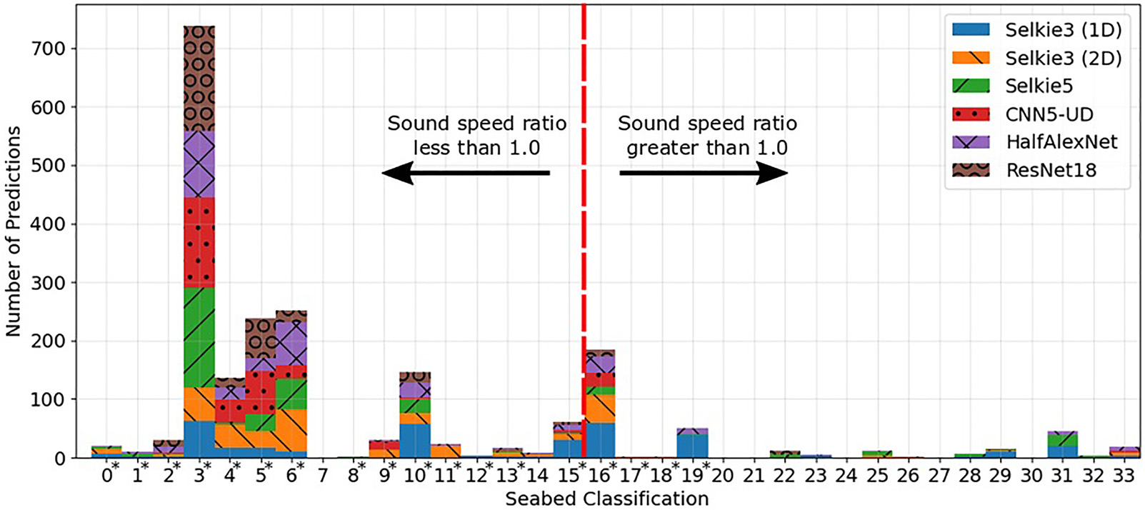
Merchant ship-radiated noise, recorded on a single receiver in the 360–1100 Hz frequency band over 20 min, is employed for seabed classification using an ensemble of deep learning (DL) algorithms. Five different convolutional neural network architectures and one residual neural network are trained on synthetic data generated using 34 seabed types, which span from soft-muddy to hard-sandy environments. The accuracy of all of the networks using fivefold cross-validation was above 97%. Furthermore, the impact of the sound speed and water depth mismatch on the predictions is evaluated using five simulated test cases, where the deeper and more complex architectures proved to be more robust against this variability. In addition, to assess the generalizability performance of the ensemble DL, the networks were tested on data measured on three vertical line arrays in the Seabed Characterization Experiment in 2017, where 94% of the predictions indicated that mud over sand environments inferred in previous geoacoustic inversions for the same area were the most likely sediments. This work presents evidence that the ensemble of DL algorithms has learned how the signature of the sediments is encoded in the ship-radiated noise, providing a unified classification result when tested on data collected at-sea.
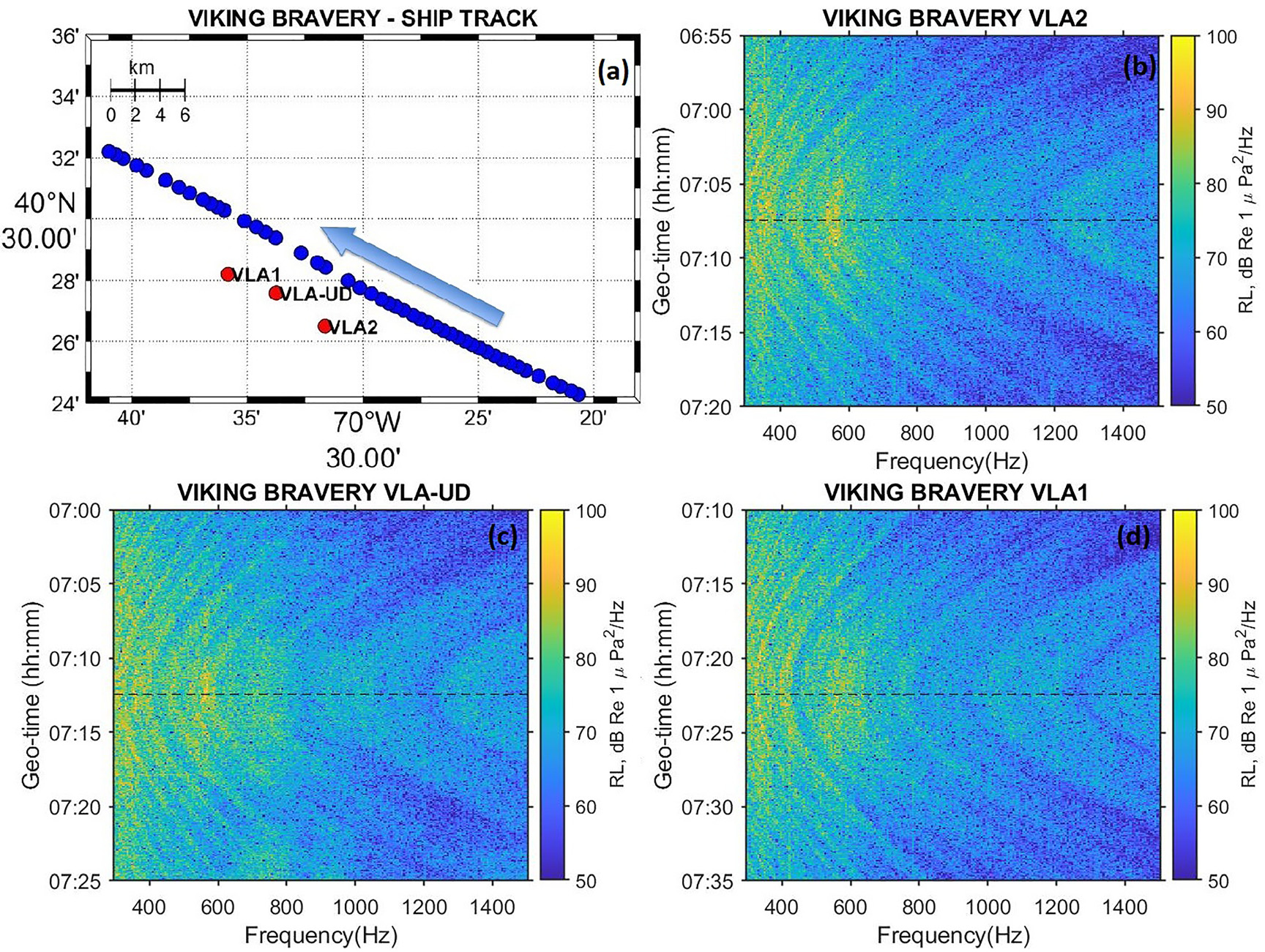
Several convolutional neural networks and and a residual neural network were applied to the measured SOO spectrograms measured during the Seabed Characterization Experiment 2017 to assess the generalizability of the networks on data collected at-sea. Classification of the 69 samples collected from the merchant ships moving next to 3 receivers located at different locations but similar depths in the SBCEX 2017 are shown below.
An ensemble of DL algorithms was implemented for seabed classification using 34 seabed types that spanned from soft-muddy to hard-sandy environments. The models were trained on 20-min normalized spectrograms over the 360–1100 Hz frequency band generated using the Wales-Heitmeyer source spectrum for a merchant ship and range independent normal-mode model ORCA. Several approaches were considered for the design of the networks by using different complexity levels in the architectures. The DL algorithms implemented in this study are as simple as a shallow 3-layer CNN (Selkie3) and as complex as a deep 18-layer ResNet (ResNet18).
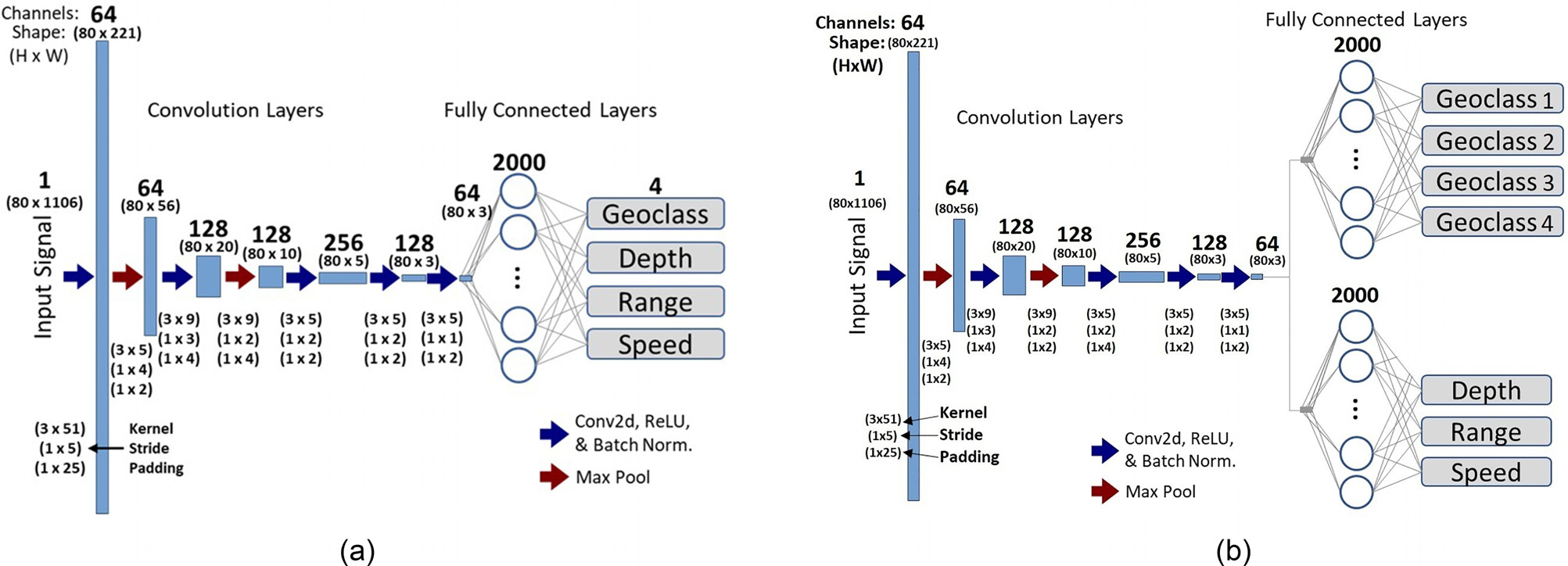
Convolutional neural networks are also used to estimate both source location and seabed type using tonals. Only regression and multi-task learning are used for this end. For networks where regression is done for all desired labels, a single fully connected layer is used prior to the output and the mean-squared error over all labels defines the loss function, as shown in Fig. 7(a). However, to accomplish multitask learning (MTL), two independent fully connected layers are used to add flexibility.
The train networks are evaluated in five tests cases with sound speed profile and seabed mismatch. Results for only regression and multi-tasks modes are shown below.
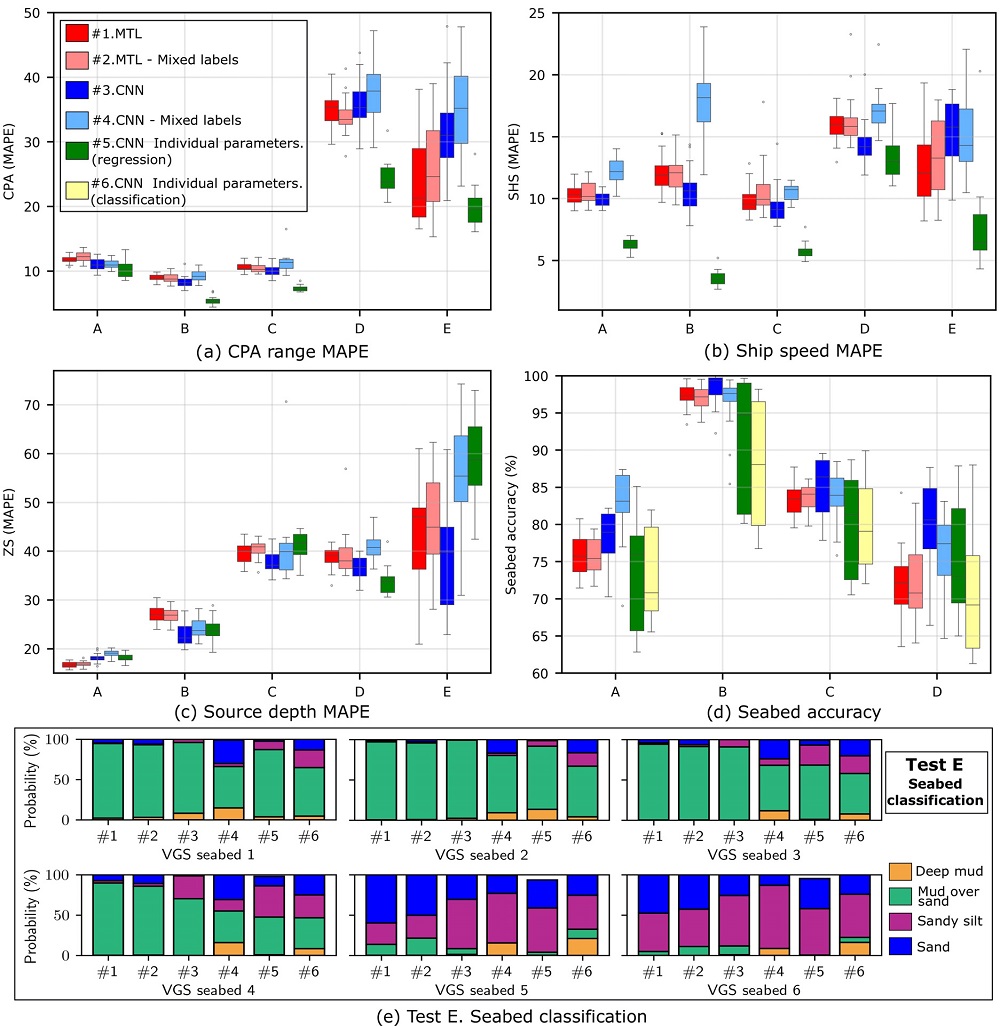
Test cases with increasing degrees of SSP mismatch showed increased error in predictions of the source labels. The trained CNNs were also applied to data simulated for seabed mismatch. This seabed mismatch, however, produced a general bias towards smaller values of all the source parameters and increased the variance in the source label predictions. These results point to the potential for seabed type characterization using MTL-CNNs and emphasize the importance of including realistic and representative seabed variations in the training data.
Related publications
-
Mohsen Badiey, Lin Wan, Christian D. Escobar-Amado, and Jhon A. Castro-Correa, . DOI: 10.1121/2.0001532. [PDF]
-
Christian D. Escobar-Amado, Tracianne B. Neilsen, Jhon A. Castro-Correa, David F. Van Komen, Mohsen Badiey, David P. Knobles, and William S. Hodgkiss. DOI: 10.1121/10.0005936. [PDF]
-
David F. Van Komen, Tracianne B. Neilsen, Daniel B. Mortenson, Mason C. Acree, David P. Knobles, Mohsen Badiey, and William S. Hodgkiss. DOI: 10.1121/10.0003502. [PDF]
-
Learning location and seabed type from a moving mid-frequency source
T. B. Neilsen, C. D. Escobar-Amado, M. C. Acree, W. S. Hodgkiss, D. F. Van Komen1, D. P. Knobles, M. Badiey, and J. Castro-Correa. DOI: 10.1121/10.0003361. [PDF]
-
David Van Komen, Tracianne B. Neilsen, David P. Knobles, and Mohsen Badiey. DOI: 10.1121/2.0001124. [PDF]
-
David F. Van Komen, Tracianne B. Neilsen, David P. Knobles, and Mohsen Badiey. DOI: 10.1121/2.0001077. [PDF]
Related Conferences
-
Seabed classification from ship-radiated noise using an ensemble deep learning
Christian D. Escobar-Amado, Mohsen Badiey, Tracianne B. Neilsen, Jhon A. Castro-Correa, and David P. Knobles. DOI: 10.1121/10.0004687