Research Statistics and modeling of internal waves
Abstract
During the Shallow Water Acoustic Experiment 2006 (SW06) conducted on the New Jersey continental shelf in the summer of 2006, detailed measurements of the ocean environment were made along a fixed reference track that was parallel to the continental shelf. The time-varying environment induced by nonlinear internal waves (NLIWs) was recorded by an array of moored thermistor chains and by X-band radars from the attending research vessels. Using a mapping technique, the three-dimensional (3D) temperature field for over a month of NLIW events is reconstructed and analyzed to provide a statistical summary of important NLIW parameters, such as the NLIW propagation speed, direction, and amplitude. The results can be used as a database for studying the NLIW generation, propagation, and fidelity of nonlinear internal wave models.
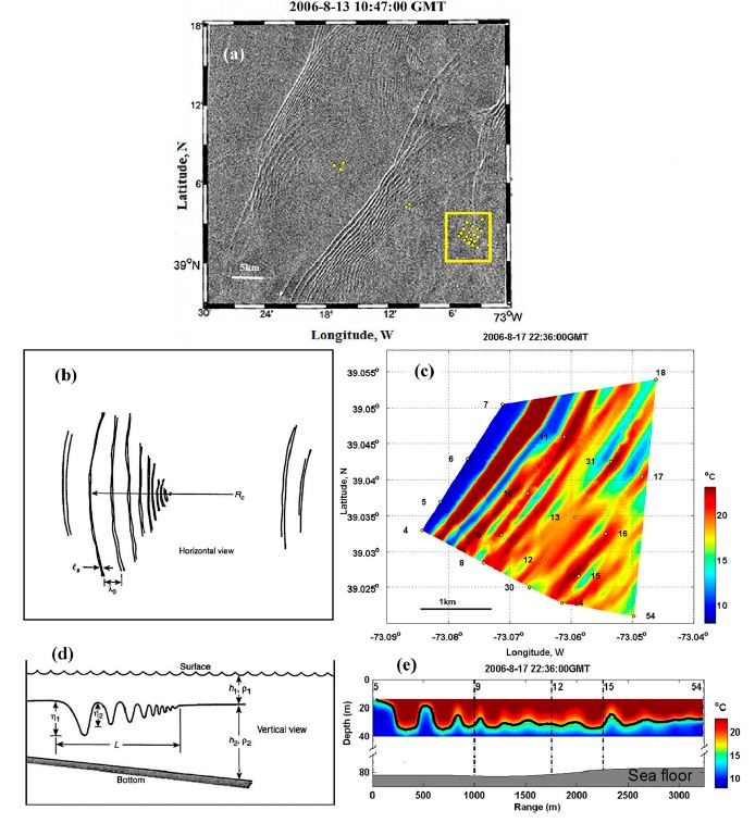
The propagation of an NLIW packet from 0422:30 to 0650:30 UTC 14 August 2006 is shown below. Panel (a) shows the top view of the reconstructed internal wave fronts (i.e., gray curves) approaching a fixed reference track (red line) at a speed of 0.68ms21. The R/V Sharp stationed at a point (green dot) right of the reference line recorded the surface radar expression of the NLIW passage [see inset in panel (b)]. Panels (c)–(j) show various elements of data collection. Vertical temperature profiles at three thermistor chains (45, 32, and 54) are shown in panels (c)–(e), respectively. The vertical dashed–dotted lines indicate the reference time of this figure at 0613:00 UTC 14 August 2006. The sound speed profiles at three points 54 (blue), 32 (red), and 45 (black) are shown in panel (f). The vertical cross section of the temperature field within the thermistor farm is shown in panel (g). The horizontal cross section of the interpolated temperature data (24m below sea surface) at three ocean patches is shown in panels (h)–(j).
We developed a statistical database from 30 recorded NLIW events during SW06. These statistical data were obtained when the NLIW packet was located inside the thermistor farm, such that the first front was close to the far edge of the farm (i.e., along points 4–7 shown for an event on 17 August 2006 in Fig. 1(c). There are eight directly measured parameters and seven derived ones. To the extent possible, we have followed Apel’s notation in choosing these parameters. The mean value of each parameter, its standard deviation, and its estimated measurement error are listed in the Table below.
| Characteristic (symbol) | Unit | Typical scale | SW06 results | Uncertainty |
|---|---|---|---|---|
| Upper layer depth $(H_1)$ | m | 5-25 | 17.6 $\pm$ 3.7 | 2.4 |
| Lower layer depth $(H_2)$ | m | 30-200 | 59.1 $\pm$ 3.7 | 2.4 |
| Direction $(\alpha)$ | ° | a. s. | 309.8 $\pm$ 13.0, 13.4 $\pm$ 8.7 | 0.2 |
| wavelength $(\lambda_0)$ | m | 100-1000 | 513.0 $\pm$ 179.8, 1525.2 | 5.0 |
| First amplitude $(\eta_1)$ | m | 0-30 | 4.9 $\pm$ 1.9, 16.8 $\pm$ 3.6 | 2.4 |
| Second amplitude $(\eta_2)$ | m | 0-30 | 4.5 $\pm$ 1.6, 14.3 $\pm$ 4.9 | 2.4 |
| Soliton width $(L_s)$ | m | 100 | 176.4 $\pm$ 58.8 | 5.0 |
| Number of solitons $(n)$ | d.u. | 1-20 | 4.9 $\pm$ 1.7 | 2.2 |
| 16.7 $\pm$ 4.3 | 4.1 | |||
| 42.0 $\pm$ 2.8 | 6.5 | |||
| Speed $(v)$ | m$\textrm{s}^{-1}$ | 0.5-1.0 | 0.8 $\pm$ 0.1 | 0.003 |
| Amplitude/upper depth $(\gamma)$ | d.u. | 0-6 | 0.4 $\pm$ 0.2 | 0.1 |
| Slope of IW faces $(K)$ | d.u. | 5-100 | 36.4 $\pm$ 24.4 | 19.0 |
| Packet length $(L)$ | km | 1-10 | 5.5 $\pm$ 1.8, 14.3 $\pm$ 2.0 | 0.02, 0.06 |
| Packet spacing $(D)$ | km | 15-40 | 12.4 $\pm$ 5.8, 34.4 $\pm$ 4.4 | 0.04, 0.11 |
| Decay constant $(\beta)$ | k$\textrm{m}^{-1}$ | 0.1-1.0 | 0.36 $\pm$ 0.33 | |
| Radius of curvature $(R_c)$ | km | 15-$\infty$ | 4.2 |
From the table, the following conclusions can be made: 1) the majority of the 30 NLIW events studied in this paper have the depth of the warm layer ($H_1$=17.6 m) and depth of the cold layer ($H_2$=59.1 m). 2) About 90% of the NLIWs propagate in the direction of 3108 with respect to true north and originate near the New Jersey shelf break. About 10% of the NLIWs propagate at approximately 108–138 with respect to true north and likely originate from the Hudson Canyon. The propagation speed of these waves (in both groups) is about 0.8 m$\textrm{s}^{-1}$. 3) The first and second soliton amplitudes in each packet during 61% of the total events indicate an amplitude decay of 0.36k$\textrm{m}^{-1}$. In some odd cases, the amplitude of the second soliton is larger than the first soliton, a peculiarity seen due to the variability in the background ocean affecting a nonlinear system. 4) The ratio of the soliton wavelength to the soliton width is about 2.91, this is comparable to the predicted ratio. 5) The average amplitude of the first soliton to the upper-layer depth ratio is 0.4. 6) The slope of the first soliton for the majority of the events in our database is about 36.4.
Related publications
-
Statistics of Nonlinear Internal Waves during the Shallow Water 2006 Experiment
Mohsen Badiey, Lin Wan1, and James F. Lynch. DOI: 10.1175/JTECH-D-15-0221.1. [PDF]
-
Three-dimensional mapping of evolving internal waves during the Shallow Water 2006 experiment
Mohsen Badiey, Lin Wan, and Aijun Song. DOI: 10.1121/1.4804945. [PDF]