Research Acoustic normal mode fluctuation statistics
Abstract
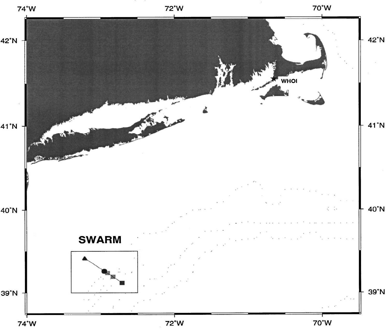
In order to understand the fluctuations imposed upon low frequency 50 to 500 Hz! acoustic signals due to coastal internal waves, a large multilaboratory, multidisciplinary experiment was performed in the Mid-Atlantic Bight in the summer of 1995. This experiment featured the most complete set of environmental measurements especially physical oceanography and geology made to date in support of a coastal acoustics study. This support enabled the correlation of acoustic fluctuations to clearly observed ocean processes, especially those associated with the internal wave field. More specifically, a 16 element WHOI vertical line array WVLA! was moored in 70 m of water off the New Jersey coast. Tomography sources of 224 Hz and 400 Hz were moored 32 km directly shoreward of this array, such that an acoustic path was constructed that was anti-parallel to the primary, onshore propagation direction for shelf generated internal wave solitons. These nonlinear internal waves, produced in packets as the tide shifts from ebb to flood, produce strong semidiurnal effects on the acoustic signals at our measurement location. Specifically, the internal waves in the acoustic waveguide cause significant coupling of energy between the propagating acoustic modes, resulting in broadband fluctuations in modal intensity, travel-time, and temporal coherence. The strong correlations between the environmental parameters and the internal wave field include an interesting sensitivity of the spread of an acoustic pulse to solitons near the receiver.
Figure 2 shows a typical set of 400-Hz pulse-compressed arrivals for the 16 hydrophones at the WVLA. The term "typical" is used rather loosely here, as the scattering from internal waves in the waveguide causes significant temporal variability in the individual hydrophone arrivals. What is typical here is that a set of arrivals generally consists of an early packet of energy with a mode one amplitude and phase depth dependence followed by a signal of about about 100-ms duration having "mixed mode" characteristics.
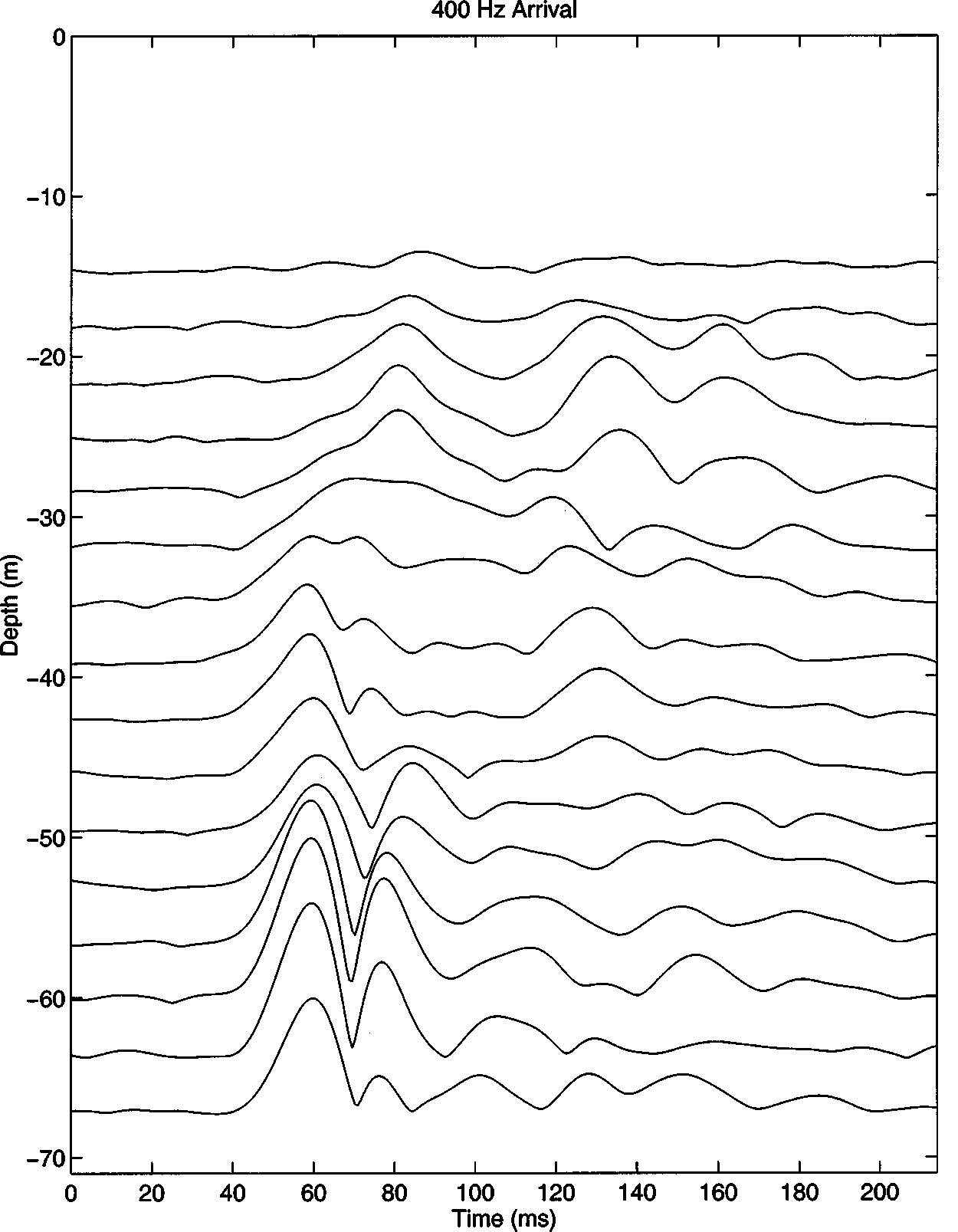
The 224-Hz arrivals are similar, but the narrower bandwidth 16 Hz yields a broader pulse width (60 ms). The 224-Hz source produced a 63 digit, phase-modulated signal with a digit length of 14 cycles, with period 3.9375 s per sequence. The sequence was repeated 30 times during each transmission, for a total transmission time of 118.125 s. The transmissions were repeated every 5 min, starting on the hour. They were received at the WVLA about 22.5 s later. The modal analysis of 400-Hz acoustic arrivals at the WVLA begins by treating the acoustic signal at each hydrophone as a sum of vertical modes:
$$p_h(t) = \sum_{n=1}^N A^n(t) \phi_n(z_h)$$
where $\phi_n(z)$ is the modal pressure depth function, $A_n(t)$ is the mode coefficient, and $z_h$ is the depth of the hth hydrophone. The number of propagating normal modes, $N$, as well as the mode shapes themselves are frequency dependent.
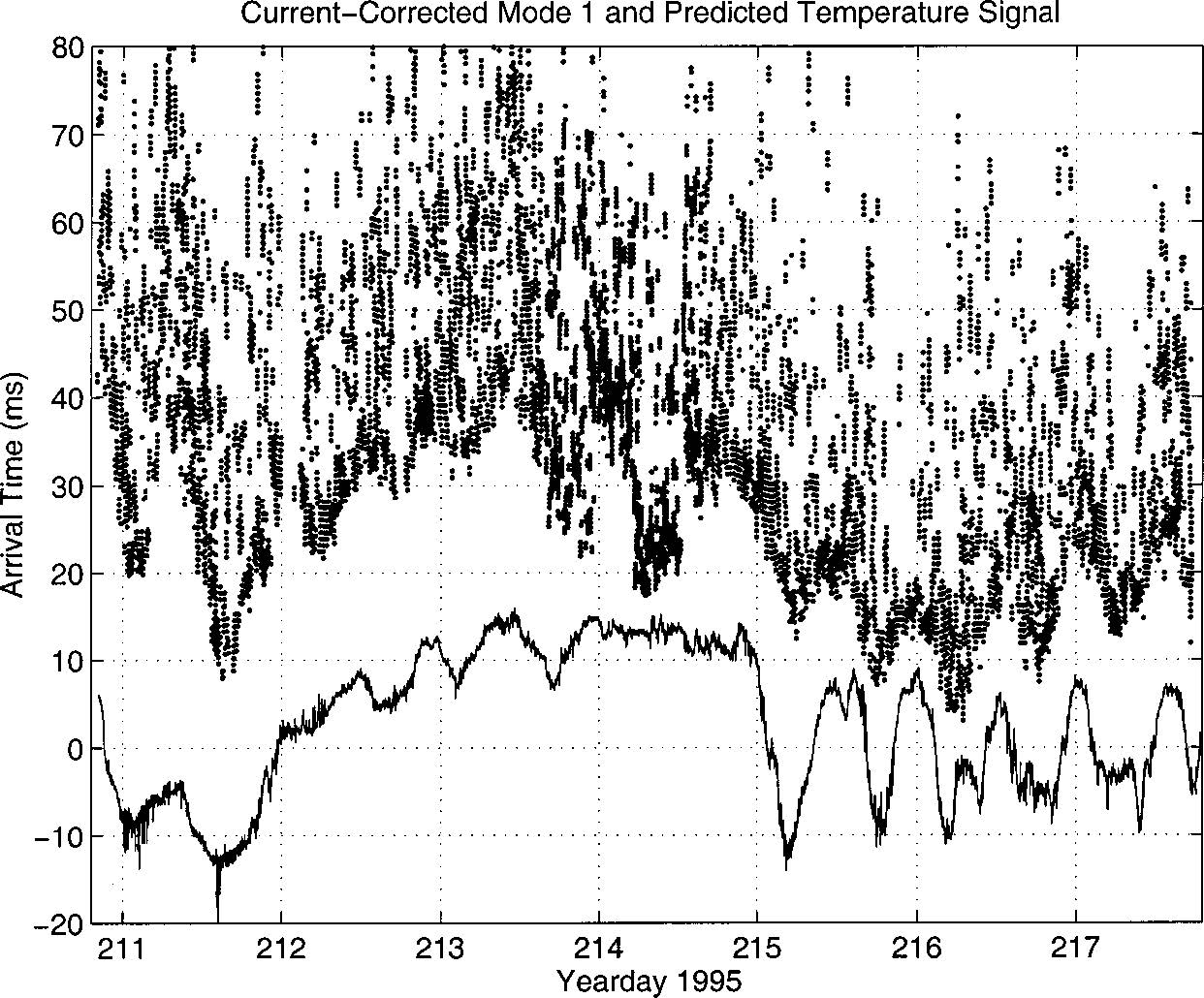
The "current-corrected" distribution of SWARM mode one peak arrival times, which is our cleanest data set for the modes, is shown in Fig. 3. The arrivals have a fairly sharp leading edge; there is little or no indication of negatively biased peaks. [The current-correction to travel-time is derived from a bottom moored current meter near the WVLA. Specifically, the predicted travel-time fluctuations order 63 ms obtained from applying the measured barotropic (depth independent) currents (predominantly M2 tidal, i.e., the strong 12.42-h period semidiurnal tidal component) to the entire acoustic path were subtracted from raw peak arrival times.] The mode one wander, as seen in Fig. 3, is substantial, and a good portion of it can be correlated with temperature fluctuations in the vicinity of the WVLA. These fluctuations were logged in thermistor records from the WVLA and three dedicated thermistor strings moored in a cluster 4.5 km shoreward of the WVLA. The solid curve in Fig. 3 is obtained by using the average change in sound speed seen at seven of these thermistors to calculate travel-time variations.
Acoustic normal mode arrival time spread and bias, and the modal intensities and decorrelations times measured in the 1995 SWARM experiment show distinct M2 tidal period fluctuations. These are highly correlated to the passage of trains of solitons between the source and receiver. A particular interesting correlation was that of the maximum modal pulse spread with solitons near the acoustic receiver. Although we have not shown it here, there are no other oceanic or bottom acoustic phenomena which can create this same M2 type of signal in our data, so we can reasonably state that these effects are due to internal tide solibores.
Related publications
-
Acoustic normal mode fluctuation statistics in the 1995 SWARM internal wave scattering experiment
John Apel, Mohsen Badiey, Ching-sang Chiu, Steve Finette, Marshall Orr, Bruce Pasewark, Alton Turgot, and Steve Wolf, and Dirk Tielbuerger. DOI: 10.1121/1.428563. [PDF]