Research Inversion using low frequency acoustic data
Abstract
When using geoacoustic inversion methods, one objective function may not result in a unique solution of the inversion problem because of the ambiguity among the unknown parameters. This paper utilizes acoustic normal mode dispersion curves, mode shapes, and modal-based longitudinal horizontal coherence to define a three-objective optimization problem for geoacoustic parameter estimation. This inversion scheme is applied to long-range combustive sound source data obtained from L-shaped arrays deployed on the New Jersey continental shelf in the summer of 2006. Based on the sub-bottom layering structure from the Compressed High-Intensity Radiated Pulse reflection survey at the experimental site, a two-layer (sand ridge overlaying a half-space basement) rangeindependent sediment model is utilized. The ambiguities of the sound speed, density, and depth of the sand ridge layer are partially removed by minimizing these objective functions. The inverted seabed sound speed over a frequency range of 15–170 Hz is comparable to the ones from direct measurements and other inversion methods in the same general area. The inverted seabed attenuation shows a nonlinear frequency dependence expressed as $\alpha_b$=0.26$f^{1.55}$ (dB/m) from 50 to 500 Hz or $\alpha_b$=0.32$f^{1.65}$ (dB/m) from 50 to 250 Hz, where $f$ is in kHz.
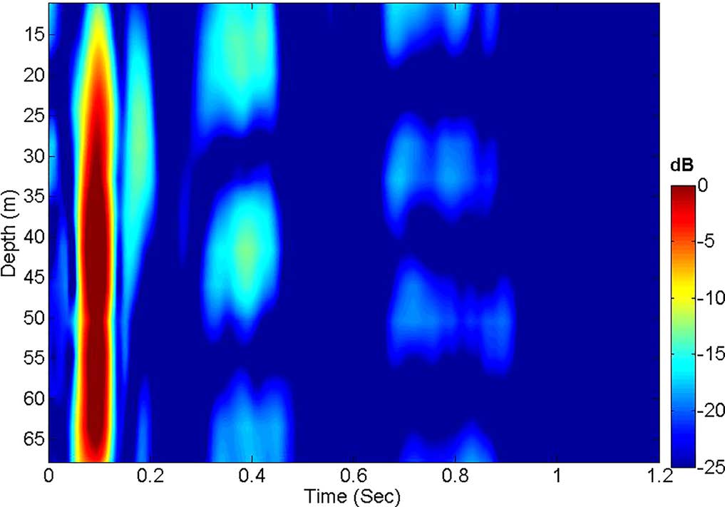
The acoustic normal modes can be identified using the CSS signal from long-range sound propagation. The received acoustic intensity (dB relative to the maximum value) of the VLA portion of SWAMI 52, at a range of 16.33 km when the CSS depth is 50 m, as shown below.
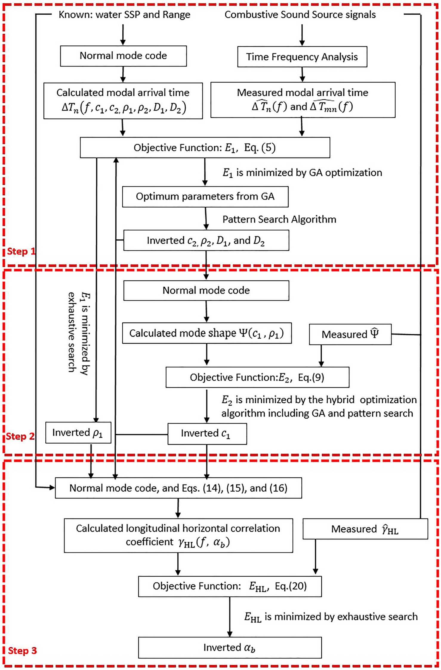
The objective function used for inversion is defined by:
$$E_1(\textbf{x})=\sum_{f} \left( \sum_{n} \left( \Delta T_n(f,\textbf{x}) - \Delta \hat{T}_n(f) \right)^2 + \sum_{m,n(m \neq n)} \left( \Delta T_{nm}(f,\textbf{x}) - \Delta \hat{T}_{nm}(f) \right)^2\right)$$
where $\Delta T_n$ is the arrival time for the mode $n$ and $\textbf{x} = [c_1, c_2, \rho_1, \rho_2, D_1, D_2]$, sound speeds, densities and depths of the water column and the first layer of sediment.
The estimation process using this hybrid optimization algorithm is shown below as Step 1. It is noted that the seabed attenuation ($\alpha_b$) is not considered as a parameter to be inverted in this first step. Because the group velocity does not depend on the seabed attenuation, an estimate for its values cannot be obtained in Step 1.
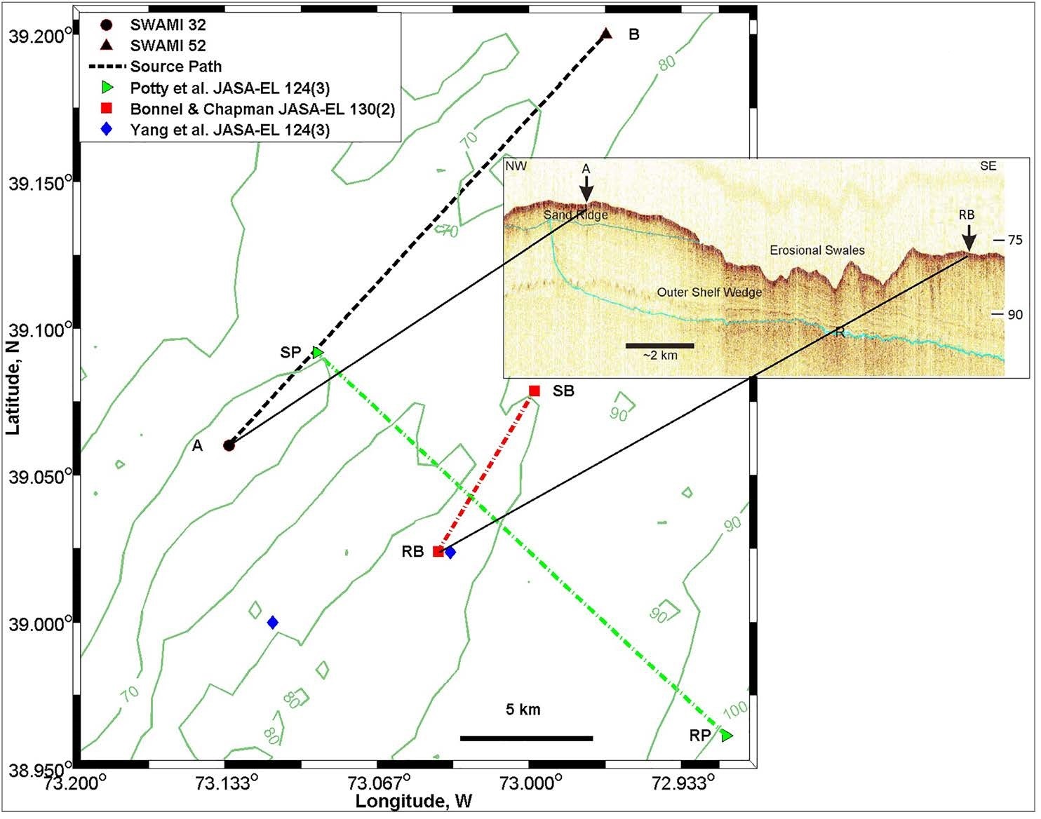
Seabed geoacoustic parameter values at the SW06 experimental site are estimated by a three-objective inversion scheme, which involves the dispersion characteristics of broadband signals, mode shapes of the acoustic normal mode, and the longitudinal horizontal coherence of the received acoustic field. Over the frequency range of 15–170Hz, the sound speed and density in the half-space basement are 1730.0 m/s and 1844.0 kg/$m^3$, respectively. The sound speed and density of the sand ridge are correlated to determine the modal arrival time difference.
Related publications
-
Lin Wan, Mohsen Badiey, and David Knobles. DOI: 10.1121/1.4962558. [PDF]