Research Inversion using airgun signals
Abstract
When using geoacoustic inversion methods, one objective function may not result in a unique solution of the inversion problem because of the ambiguity among the unknown parameters. This paper utilizes acoustic normal mode dispersion curves, mode shapes, and modal-based longitudinal horizontal coherence to define a three-objective optimization problem for geoacoustic parameter estimation. This inversion scheme is applied to long-range combustive sound source data obtained from L-shaped arrays deployed on the New Jersey continental shelf in the summer of 2006. Based on the sub-bottom layering structure from the Compressed High-Intensity Radiated Pulse reflection survey at the experimental site, a two-layer (sand ridge overlaying a half-space basement) rangeindependent sediment model is utilized. The ambiguities of the sound speed, density, and depth of the sand ridge layer are partially removed by minimizing these objective functions. The inverted seabed sound speed over a frequency range of 15–170 Hz is comparable to the ones from direct measurements and other inversion methods in the same general area. The inverted seabed attenuation shows a nonlinear frequency dependence expressed as $\alpha_b$=0.26$f^{1.55}$ (dB/m) from 50 to 500 Hz or $\alpha_b$=0.32$f^{1.65}$ (dB/m) from 50 to 250 Hz, where $f$ is in kHz.
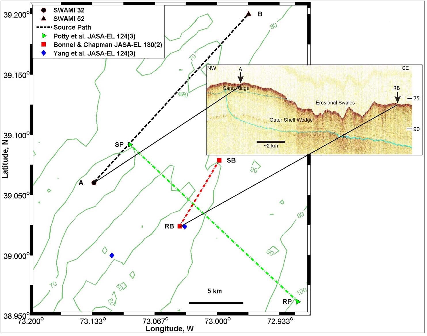
The data used in this paper were recorded in a sub-experiment between 19:00 and 20:00 GMT on August 4, 1995. The data were collected by a Woods Hole Oceanographic Institution (WHOI, Woods Hole, MA, USA) VLA with 16 hydrophones evenly spaced at 3.5 m from 14.9 to 67.4 m below the sea surface. The data were generated by an airgun source at 12 m below the sea surface and 15 km from the receiving array. The airgun source was fired at a rate of 1 min between shots. The water depth along the source–receiver track was almost constant around 72 m.
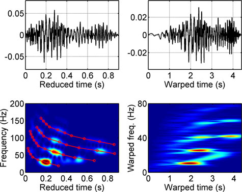
The received airgun signal (upper left) is transformed to a warped signal (upper right). Its representation in thewarped time-frequency domain is shown in the bottom-right panelwhere thewarped modes are separated. The resolved modes are then filtered and unwarped to the original time domain using $w^{−1}(t)$ to obtain the mode spectra and dispersion curves. The arrival time is obtained by the known source–receiver distance and the extracted group speed. The spectrogram of the original signal is shown in the bottom-left panel. For this focusing event four modes were extracted that cover the frequency band 20–160 Hz.
The inversion results for the seven defocusing and seven focusing events are listed in the Table, which give the overview of the inversion results of the estimated parameters. The estimated sediment sound speed and the thickness for the defocusing events are all smaller than those for the focusing events. The variation of the estimated sediment sound speeds within the defocusing events is larger than that within the focusing events.
| Event\Parameters | $c_{p1}\ (m/s)$ | $H\ (m)$ | $\rho_1\ (kg/m^3)*10^3$ | $dt\ (s)$ |
|---|---|---|---|---|
| W1168 | 1690 | 46.8 | 1.05 | -0.109 |
| W1169 | 1631 | 35.5 | 1.22 | -0.102 |
| W1170 | 1716 | 63.3 | 1.03 | -0.132 |
| W1171 | 1694 | 56.3 | 1.10 | -0.115 |
| W1172 | 1667 | 48.6 | 1.13 | -0.123 |
| W1173 | 1679 | 66.4 | 1.09 | -0.122 |
| W1174 | 1665 | 64.5 | 1.07 | -0.106 |
| Mean | 1677 | 54.5 | 1.10 | -0.116 |
| Std | 24.9 | 10.5 | 0.60 | -0.010 |
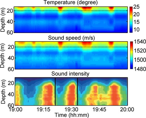
The results of the analysis indicate that the variation in the sound propagation environment has a strong impact on the modal behavior and dispersion structure. The subsequent effects on the estimation of geoacoustic parameters are investigated by inverting arrival times of the dispersed modes from 14 data sets within a cycle of the sound intensity fluctuation caused by internal waves. The inversion results for the events within each type are similar with a small standard deviation from the mean.
Related publications
-
Geoacoustic Inversion of Airgun Data Under Influence of Internal Waves
Hefeng Dong, Mohsen Badiey, and N. Ross Chapman. DOI: 10.1109/JOE.2016.2611763. [PDF]