Research Study of the azimuthal and temporal sound fluctuations
Abstract
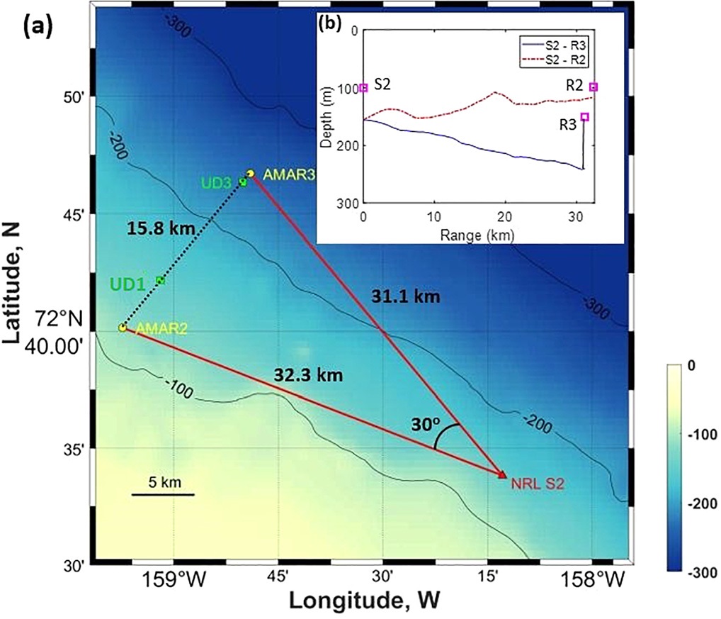
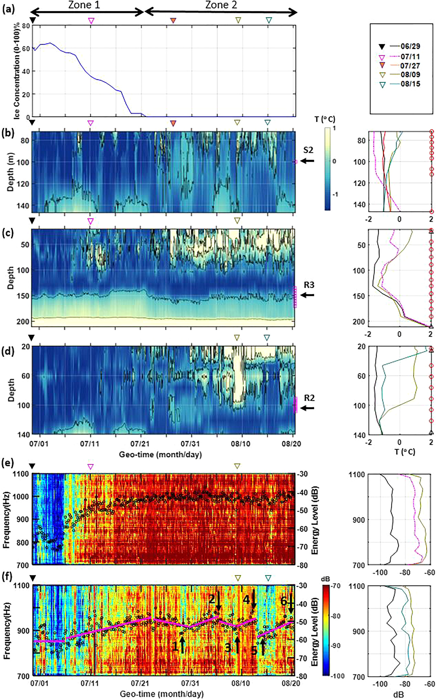
The Shallow Water Canada Basin Acoustic Propagation Experiment was conducted on the Chukchi Sea continental shelf from October 2016 to November 2017. The experimental goals were to access (1) long-range (basin-scale) and (2) short-range (shallow-water) spatial and temporal energy variation. This letter focuses on a 20-dB energy change of acoustic signals in the frequency band 700–1100 Hz from June to August 2017 occurring along two shallow-water tracks from a common source, correlated with the occurrence of an oceanographic event in the top 150-m water column due to a Pacific Water outflow from the Bering Sea and retreat of the Marginal Ice Zone.
The acoustic source S2, deployed on the continental shelf, transmitted linear frequency modulated (LFM) signals in two frequency bands: (1) 700–1100 Hz and (2) 1.5–4 kHz. The S2 source broadcasted down sweeping LFM signals with duration of 2 s for 12 min every 4 h, every day of the year as shown in Figg. 2. The acoustic energy of each pulse is calculated using $E(T_g)=\int_{f_1}^{f_2} E_0(f,T_g) \, df$. where $f_1$ and $f_2$ are the lower (700 Hz) and upper (1100 Hz) frequency limits of the signal. $E_0(f, T_g)$ is the energy spectral density as a function of frequency at geotime $T_g$. The acoustic energy is obtained by integrating $E_0$ over the frequency band (700–1100Hz).
The fluctuation of acoustic signals in the dynamic shallow water waveguide are studied calculating the correlation coefficient as a function of lag time in the same manner as shown in Refs. 10 and 11. The correlation coefficient is obtained by the equation:
$\rho(\Delta T, \tau)=\frac{\int_{0}^{\Delta T} p_1(t)p_1(t+\tau) \, dt}{\sqrt{\int_{0}^{\Delta T} p^2_1(t) \, dt \times p^2_1(t+\tau) \, dt}}$
where $\Delta T$ is the integration time, $\tau$ is the time lag, $p_1(t)$ is the reference signal received at time $t$, and $p_1(t+\tau)$ is the received signal with a time lag $\tau$.
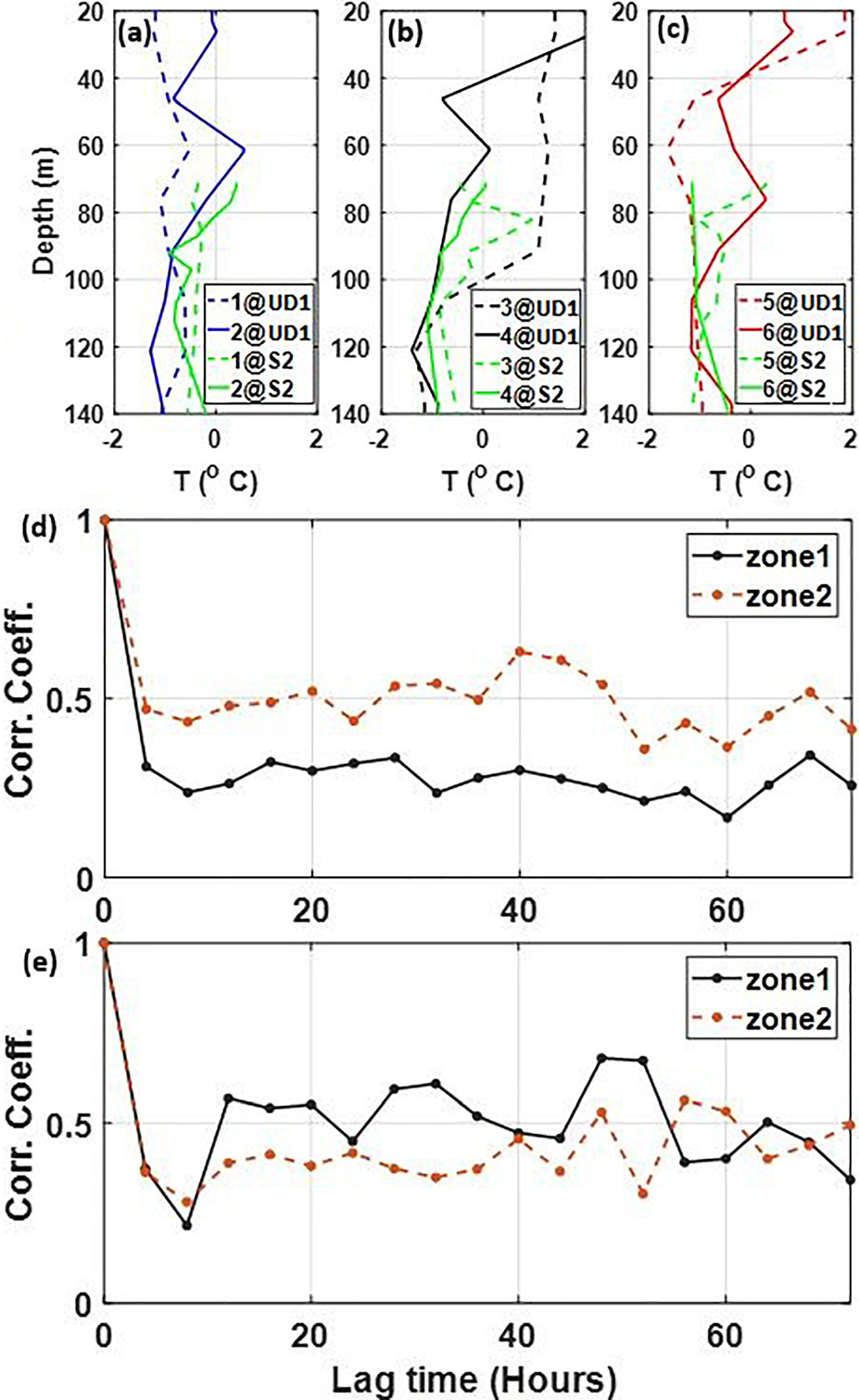
Figure 3 demonstrates higher correlation coefficient for zone 2 (ice-free) than zone 1 (60% ice coverage) along the S2-R3 track, because the effect of the fluctuations from the sea surface and bottom were mitigated due to the formation of strong sound duct in zone 2. In zone 1, the temperature profile above 120m shows a well-mixed layer, causing acoustic energy loss due to interaction with the surface ice. Figure 3(e) shows smaller correlation coefficients for zone 2 along the S2-R2 track, which could be due to the changes in bathymetry between source and receiver causing more bottom interaction of the acoustic signal.
Related publications
-
Mohsen Badiey, Lin Wan, Sean Pecknold, and Altan Turgut. DOI: 10.1121/1.5141373. [PDF]
Related conferences
-
Mohsen Badiey, Lin Wan, Sean Pecknold, and Altan Turgut. DOI: 10.1121/1.5136519
-
Mohsen Badiey, Lin Wan, Sean Pecknold, and Altan Turgut. DOI: 10.1121/1.5136609
-
Mohsen Badiey, Ying-Tsong Lin, Sean Pecknold, Megan S Ballard, Jason D Sagers, Altan Turgut, John A Colosi, Peter F Worcester, Mathew Dzieciuch. DOI: 10.1121/1.5136609
-
Mohsen Badiey, Lin Wan, John A. Goff. DOI: 10.1121/1.5035881
-
Azimuthal dependence of sound propagation due to seabed variability in shallow water
Mohsen Badiey, Lin Wan, Justin Eickmeier, David P. Knobles, and Preston S. Wilson. DOI: 10.1121/1.5014354