Derivations

As we will be interested in motion in one direction, say X direction, we can forget that our spacetime is 4-dimensional and consider only two dimensions: one spatial dimension and one time dimension. The simplest two-dimensional space-time is a two-dimensional Euclidean space , so that a given observer can parametrize it with two real numbers, saying what is the time and position of a given instance in his reference frame. Another observer will, in general, assign a different pair of numbers to the same instance, say and . For each observer, however, the assignment of a pair of numbers to a point in spacetime is 1-1, that is for each point in spacetime there exists exactly one pair of numbers (t and x) assigned to it by a given observer, and vice versa -- a given observer can show exactly one point in spacetime corresponding to t and x observed by him. So if we have two observers, the time and space coordinates observed by one of them will be a 1-1 function of the time and space coordinates observed by the other. This can be symbolically written in the following form:

If we assure that the point (0,0) for the first observer corresponds to the point (0,0) for the second one [1] then the simplest nontrivial function will be the linear one, that is:

where for i,j = 1,2.

The last expression written in matrix notation will take the form:

 

The aim is to find specific form of the matrix entries as functions of v. The physical assumption is that the numbers depend only on the relative velocity of the observers, and if the velocity is 0 they constitute a unit matrix, i.e. if the observers do not move with respect to each other, they label the spacetime in the same way. Moreover, it is reasonable to assume that if the observer A perceives B moving at the velocity v then B perceives A moving at the velocity -v. Additionally we assume that space is isotropic, that is if both observers switch the space labeling, i.e. and , the matrix does not change. Obviously, the velocity perceived by each of observers will change to the opposite; that is we have:

which gives us

If we compare the last expression with the formula (2.1), we can conclude that

 

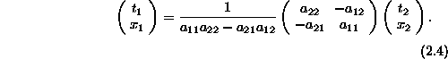
To compute the velocity of the first observer with respect to the second one we take

then, as the reader can convince himself looking at the figure 1, the velocity of the first observer with respect to the second one will be , which, since

is

 

 
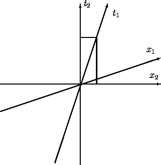
Figure 1: This figure shows how to compute the velocity of the first observer with respect to the second one . We have to take two different points corresponding to the same position for the first observer (we have chosen (0,0) and (1,0)), and then compute which is as we start from (0,0). 

To compute the velocity of the second observer with respect to the first one ( ) in terms of matrix elements , we take the inverse of the relation (2.1):

 

Substituting

to (2.4) we get

which, by the same argument as before, gives us

 

As , we get by (2.3) and (2.5)

which leads to

By (2.3), gives v=0. In this case becomes a unit matrix. When the observers move at nonzero velocity w.r. to each other , so

 

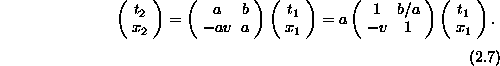
If we define and , then using (2.5), (2.6) and we can rewrite (2.1) as:

 

So far we have reduced the problem of finding 4 functions , to the problem of finding two functions a(v) and b(v). To proceed further, consider a third observer, who moves with respect to the first one at the velocity v'. He will also move with respect to the second observer. Let . As the relation (2.7) is true for any pair of observers we can write:

 

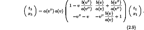
and

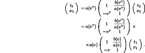
The last expression, after multiplication of matrices, yields:

 

The expressions (2.8) and (2.9) represent the same transformation, therefore the matrix entries have to be the same. In particular if we compare diagonal elements, we get

which gives us

or [2]

 

What we have in (2.10), is that the quantity

 

is the same for any v, as in (2.10) v and v'' are arbitrary. That is , independent on velocity. This is a fundamental constant, that has to be determined experimentally.

Thus, we can write b(v) as . Then (2.7) becomes:

 

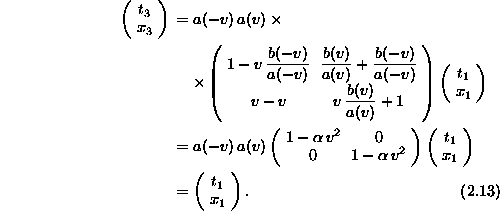
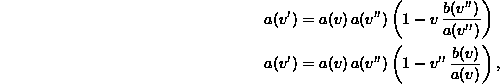
and the only function that remains to be established is a(v). To find the form of a(v), we observe, that if the third observer moves with respect to the second one at the velocity -v, where v is the velocity at which the second observer moves with respect to the first one, then the third observer is at rest with respect to the first one. That is, by (2.9) and (2.11)

 

Using (2.2) we can write (2.13) in the form:

As the last expression has to be true for any and , we find that

Apparently we have two choices for a: . However, to be consistent with the case when v=0, where becomes a unit matrix, we are bound to take the + sign,

 

So finally the transformation becomes:

 

Or

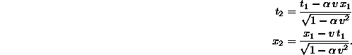
If we can write , where c is a real number, that has a dimension of velocity; (2.15) takes then the form of the famous Lorentz transformation, where the constant c is now interpreted as a speed of light, or the upper limit of speed of an observer perceived by another one. For we recover Galilean transformation. When we get the so called elliptical rotation; if we rescale the time coordinate to make , and then substitute the transformation (2.15) becomes a simple rotation by an angle in the T,X plane.