
Introduction
This chapter discusses several time transfer scenarios involving planetary and deep space orbiters, landers and probes. While the objective is to synchronize the clock in these vehicles to Earth, this function is often integrated with the navigation functions [STA 02, GIF 06]. This chapter relies heavily on the material of the preceding chapter and on general knowledge of mathematics and physics principles. While the general relativistic effects described in the previous chapter are always present to some degree, they will be neglected in this chapter.
The first scenario, which involves a geosynchronous satellite, is not really a space mission, since it describes time transfer between national laboratories on Earth. However, the means described could be used for time synchronization on the Moon or on other planets where distances are relatively snall and signal/noise ratios (SNR) are relatively large.
The second scenario involves time synchroniztion for Mars orbiters and landers. The means described use the internationally standardized Proximity-1 protocol. NASA/JPL operational procedures now provide navigation and time transfer direct from Earth via the JPL Deep Space Network (DSN). As the number of vehicles near and on Mars grows over time, DSN resources may become prohibitively expensive. We discuss an alternative where one or more Mars vehicles are synchronized from Earth and then they provide time transfer for the other Mars vehicles.
The third scenario involves navigation and time transfer from Earth to space vehicles. The DSN has recently transitioned from a multiple-subcarrier ranging system to a system using a pseudo-random signal. The technique requires considerable resources which are impractical for space vehicles, but does not provide precision time to the space vehicle. The Parting Shots section describes a method with which this might be achieved.
Time Transfer Between Earth Stations
Early in the history of time transfer between national laboratories the only way to synchronize cesium clock ensembles was to fly a portable cesium clock from one site to another. While cesium clocks typically have batteries, the battery charge lasts only a few minutes long enough for the backup generator to kick in. For transport over intercontinental distances they required a first class seat and heavy duty deep-discharge battery. It is very unlikely that airlines would permit that today.
In recent times the LORAN-C longwave radio and later GPS satellite navigation systems have become available and the flying clocks have been grounded. These means provide accuracies to the microsecond for LORAN-C and to the nanosecond for GPS. However, GPS is only a common-view system and does not provide a two-way capability. In particular, a method is needed for time transfer between stations that does not involve a flywheel clock in the satellite.
The solution developed by NIST [HAN 89] and later refined by USNO [LAN 92] is called Two-Way Satelite Time and Frequency Transfer (TWSTFT) [KIR 91]. It uses a common-view geosynchronous satellite capable of two-way operation with very small antenna terminal (VSAT) Earth stations and a digital modem specially designed for time transfer service. In operation each station sends an on-time pulse together with ancillary information via the satellite to the other station. After compensation for various propagation effects, the time of each station relative to the other can be determined to 100 ps or better.
The VSAT terminals and geosynchrounous satellite operate at Ku band, 14 GHz Earth to satellite and 12-GHz satellite to Earth. The transmitter power is typically 10 W and the antenna diameter 1-2 m. The RF upconverter and downconverter operate with 70-MHz IF and a digital modem. Equipment with these charateristics is common in the satellite comunications community.
What makes the TWSTFT application unique is a special digital modem first implemented as the Hartl/Mitrex modem [HAN 89] and later refined by USNO [LAN 92]. It uses the 1-Hz (PPS) and 5-MHz signals generated by a cesium clock. The PPS signal is used as a precision time tag for transmission of one station to the other, while the 5-MHz signal is multiplied to 25 MHz and used to drive A/D converts and timing signals used in the modem.
The heart of the modem is a pseudo-random (PR) sequence generated by a linear-feedback shift register (LFSR). Devices like these are widely employed in digital communication systems. The USNO modem uses a 12-stage LFSR which generates a sequence of 212 – 1 = 4095 bits (more properly called chips) with a uniquely powerful autocorrelation function together with a very low crosscorrelation function. This makes the LFSR ideally suited for time transfer applications.
In the USNO design each 4095-chip PR sequence is interpreted as one bit in a word of 32 bits. Nineteen words are bi-phase modulated on a carrier frequency of 4095 x 32 x 19 = 2.489760 Mbps, which is appropriate for a commercial TV satellite transponder. A binary one is transmitted in the upright phase, while a binary zero is transmitted in the inverted phase. The resulting signal consists of a 32 x 19 = 608 Hz data stream.
The data stream begins with the on-time tag followed by the time of day, station identifier and ancillary data. The on-time tag consists of 16 bits of zero followed by 16 bits of one, which cannot be duplicated by legitimate data.
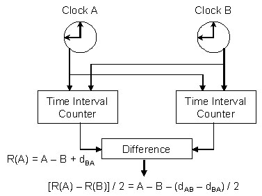
As shown in the figure, each station includes a time interval counter which is initialized at zero when a station transmits the on-time tag to the other station. Upon receiving the on-time tag, a station stops its counter and sends its value to the other station in the next second. Upon completion of two rounds, each station subtracts the value received from the other statino from its own value. As shown in the figure, the offset between the stations can be easily computed; in fact, this method is a variation of that used by NTP.
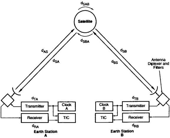
The success of this method depends on accurate calibration of residual delays. In the above figure dTA includes components due to cables, modem and RF equipment. The dAS includes includes components of the ionosphere and troposphere, while dSAB includeds the effects of the satellite transponder and related RF equipment. In practice, every attempt is made to keep the signal paths symmetric so these delays cancel out
In addition, an adjustment called the Sagnac effect must be used to compensate for the motion of the satellite during the time of passage between one station and the other. The following figure shows how this is done.
Consider the geometrical figure formed by the line segments connecting the satellit, each Earth station and the center of the Earth geoid as the path SACBS. Then form the projection of this figure on the Earth equator and compute the area A of the projection in km2. The Sagnac correction is d = 2Aω / c2, where ω is the angular velocity of the Earth in rad/s and c is the velocity of light in km/s.
In practice a number of exhanges are made over a period of minutes and the counter values averaged to refine the measurements. In this way the offsets between stations can be determined to within 100 ps. In addition, a number of stations can participate where one of them polls the others in turn so all stations can measure their laboratory offsets relative to the others in one session. At one time NIST and USNO participated in these measurements three times a week.
Time Transfer for Earth Satellites
This section describes a method for time tranfer from Earth to an orbiting satellite. Accuracies within 5 μs were demonstrated in a NASA Shuttle mission using the Tracking and Data Relay Satellite System (TDRSS). TDRSS supports multiple, simultaneous, near-Earth space missions using several GEO satellites operating at S and Ku bands. The satellites use wideband, quasi-linear transponders, often called "bent pipes".
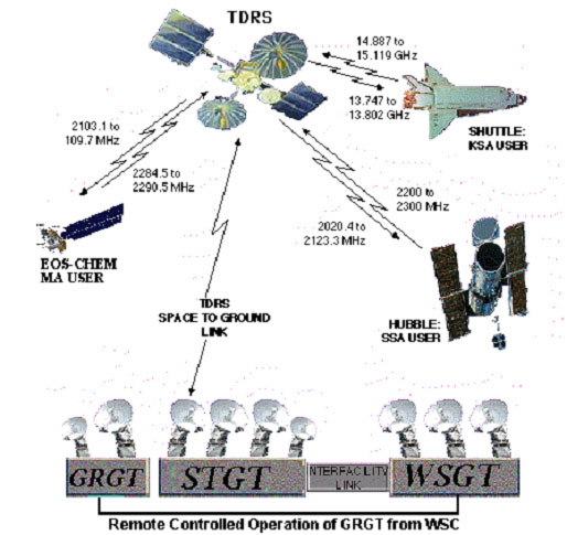
The figure above shows Earth stations operated from White Sands, NM, a TDRSS satellite and the Shuttle. Uplink S-band signals from White Sands are translated by TDRSS to Ku band and downlinked to the Shuttle. These signals are immediately translated to another Ku band frequency, uplinked to TDRSS, translated to S band and downlinked to White Sands. There is no buffering or delay; the entire process is done ar RF.
For time transfer puposes the White Sands uplink signal is modulated by a PR ranging signal similar to the TWSTFT signal. At regular intervals the uplink equipment inserts a pulse in the ranging signal and saves the current time T1. The pulse is synchronized by precision means to UTC. Equipment onboard the Shuttle captures the pulse and saves the current onboard clock T2. When the pulse is receive at White Snads, the current time is saved in T3. White Sands now calculates T4, the time the pulse arrived at the Shuttle and uplinks this value in the telemetry stream. The Shuttle onboad clock correction is T4 – T2 with accuracy limited prinmarily by the White Sands station clocj.
In this design the time for the pulse to leave White Sands and come back takes two roundtrips between on and near Earth and GEO, which is about 540 ms. As in the TWSTFT technique, the paths are symmetric and the various delays, except the Sagnac effect, generally cancel out.
At Whits Sands T4 is calculated as
T4 = T1 + (T3 – T1) / 2 + dS,
where dS is the Sagnac effect due to the rotation of the Earth during the roundtrip time T3 – T1. Unlike the TWSTFT technique where the satellite is stationary at GEO, the Shuttle is moving along its orbit. However, the time while the pulse is turned around at the Shuttle is very small, so the Sagnac effect can be calculated as in TWSTFT. Finally, the Shuttle is in LEO and moving relatively slow, so the effects of general relativity can be ignored.
Time Transfer for Satellites of the Moon and Other Planets
A good deal has been written about navigation, communiation and time transfer to planetary systems, including the Moon and its satellites [STA 05], Mars and its satellites [EDW 04, EDW 06] and deep space [GIF 06, MIL 07]. In general, there is a clear distinction between vehicles with navigation as the primary purpose, and other vehicles with primary purpose science data collection and data relay. Navigation vehicles need to precisely measure range and range rate in order to determine state vectors for other vehilces. For this purpose they need ultra stable oscillators (USO) which cost welll into six figures. While these vehicles do not need precise time transfer from a coordinated timescale such as UTC, it is natual to embed a time transfer capability in the navigation signal, as described in a later section of this chapter. In other vehicles not intended for precise navigation, time transfer can be embedded in the communications protocols such as Proximity-1 and NTP.
The first consideration is the orbits that might be involved in a planetary fleet of communication, navigation and science vehicles. A scenario for a developing Lunar navigation and communications network has been proposed in [GIF 06]. It starts with a constellation of three polar orbiters approximately 120° apart, which would support Lunar polar missions on a continuous basis. These orbiters would need a navigation capability to locate landers, as well as navigation signals that enable landers to determine surface position. Time transfer could be provided either using the Proximity-1/NTP protocol, as described in a previous sectionk or by embedding a time-tag in the ranging signal, as described in the next section.
Polar orbiters would be in view of the DSN for at least half the orbit period. Howeverf, in this configuration the orbiters would never see each other and would not support Lunar missions at lower latitudes on a continuous basis. To do this, the authors propse a three-orbiter constellation of equatorial satelllites again spaced 120° apart. In the evolved 6-orbiter network there would be frequent crosslink opportunities between the polar orbiters and equatorial orbiters. A constellation like this could be used for Mars and the other planets as well.
An orbiter with a two-hour period, for example, will scan the same surface point twice each day, once on the ascending pass, once on the descending pass. However, each pass advances 30° from the last, so a surface point might not see more passes than this. In any case, a pass is not likely to last very long - a few to ten minutes at Mars, for example. A constellation involving Moon orbiters and landers is a special case, since the Moon as seen from Earth always shows the same face. As seen from a llunar polar orbiter, the Moon appears to rotate with the same 24-hour period as Earth.
Iif multiple polar orbiters are deployed to improve the communcations and navigation coverage, they probably will not be able to communcate with each other. Some authors have proposed one or more equatorial orbiters at medium to high altitudes to provide a relay capability between orbiters and landers, especially on the far side of the Moon, which cannot be reached directly from Earth. Such a scenario is explored in the next section of this chapter.
Some briefings have suggested a relay/navigation satellite placed at the L1 Lagrange point; that is, at the Earth-Moon barycenter located about 23,000 km from the Moon surface. As shown in the figure below, there are five Lagrange points for the Earth-Moon system with Earth at the center of the orbit. All but L4 and L5 are unstable, so the position must be actively managed using spacecraft propellants.
While not found in the briefings, the L2, L4 and L5 points might be useful for relay betwen Earth and the far side of the Moon without using polar orbiters. An additional opportunity a so-called halo orbit at the L1 point is possible where the orbit plane is perpendicular to the line joining the Earth and Moon centers and the center of the orbit is at L1. This might make possible using the halo orbiter to relay between Earth and L2 without occultation by the Moon.
Some brieftings have suggested use of Earth orbit resources as a navigation and time transfer augmentation, including TDRSS and GPS. There are problems perhaps not forseen using these resources. First, the Earth satellite antennas are optimized for the Earth or Earth orbit and are useful only when the Earth orbiter is shortly before passing behind the Earth or shortly after it emerges from behind it. This issue is discussed in the next section. Second, the Earth orbiting spacecraft antenna boresight and link budget is optimized for near-Earth communication and may not be sufficient for near 300,000-km links to the Moon. To some extent this can be mitigated by a high-gain antenna at L1. If so, time transfer to L1 might be possible using TDRSS and the TDRSS method described previously. It might also be possible to use GPS in a similar manner, but only at times when the link budget permits, which might not result in continuous operation.
Time Transfer for the MARS Spacefleet
This section discusses issues involved in time transfer from one spacecraft to another using the PITS protocol described in a previous chapter. It assumes each spacecraft has the computing capacity to determine and update its current state vector.
In early 2009 NASA and the European Space Agency (ESA) have a number of orbiters and landers on Mars, including three orbiters Mars Express (MEX), Mars Reconnaissance Orbiter (MRO) and Odyssey ODY. Plans later this year are to lauch a new lander, Mars Science Laboratory (MSL). At present there are two Mars rovers (MRO), Opportunity and Spirit, and one fixed lander Phoenix (PHY), but they landers might not limve much longer. All but PHY can communicate at X band directly to Earth via the DSN, but only at very low data rates. In addition, the Mars vehicles can communicate with each other using Electra transceivers with the Proximity-1 protocol.
At present, intersatellite data and time transfer are coordinated from Earth, which requires considerable DSN resource committments in competition with other DSN missions. As the number of vehicles lurking in the Moon vicinity and in the Mars vicinity continues to grow, there is a need to provide time and data transfer directly between Moon vehicles and between Mars vehicles.
This section contains a strawman proposal that could be used with any planetary body, including Earth, the Moon and Mars. It involves a scheduling algorithm that utilizes available communications crosslink opportunities between the vehicles. The scheduling algorithm can be implemented in a flexible manner with some components on Earth and some others on space vehicles. It can evolve by gradually moving some components from Earth to the space vehicles, retaining Earth components for backup. Eventually, the vehicles would be able to determine the pass opportunities and transfer time and data from one vehicle to another possibly via a third or even fourth vehicle. It is understood that this can become rather intricate, as the vehicles move in different orbits and crosslink opportuinities may conflict.
In order to determine the feasibility of such an approach, an experiment has been implemented to simulate a projected Mars spacefleet using a constellation of satellites orbiting Earth. The reason for using Earth rather than Mars for this simulation is that Earth satellite orbit data are readily available, but Mars satellite orbit data are not. The experiment involves five Earth orbiters and one Earth lander.
ID |
Spacetrack Name | Altitude (km) | Inclination | Period (h) |
1 |
AMSAT OSCAR 40 | 800-58000 | 7.9° | 19.11 |
2 |
AMSAT ECHO | 800 | 98.1° | 1.67 |
3 |
NAVSTAR 62 | 20000 | 55.3° | 11.97 |
4 |
INTELSAT 1002 | 36000 | 0.0° | 23.93 |
5 |
NOAA 18 | 870 | 98.0° | 1.70 |
6 |
W3HCF | surface | 39.7N 75.8W |
This constellation was chosen to explore the forwarding delays and throughput of the various crosslinks between the vehicles. Vehicles 2 and 5 are typical satellites at LEO, but seldom, if ever, see each other. Vehicle 3 is a GPS satellite at MEO, while vehicle 4 is an INTELSAT communications satellite at GEO. Vehicle 6 is on the surface near Philadelphia, PA. The interesting case is vehicle 1, which has a highly eccentric orbit with apogee beyond GEO. This satellite spends most of its time loitering near apogee and zips around the Earth near perigee.
The simulator itself uses a software library available from JPL called the SPICE Toolkit. It includes an extensive set of routines to perform vector calculus, time metrology, geometric transformations and state vector processing. The library is used by JPL mission planners and scientific investigators from several institutions.
The simulator first initializes all five orbiters using the Keplerian elements from the NORAD Spacetrack database, which catalogs radar tracking data for almost all objects in Earth orbit. This establishes the initional state vector for each vehicle at a given time. Subsequently, at intervals of one minute the state vector for each vehicle is updated by integrating along the orbit.
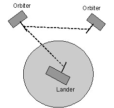
Next, a pass list is constructed which shows each pass where one vehicle can see another; i.e., only if the ray path is not occulted by Earth or by components on the spacecraft itself, as shown in the figure. A pass list entry includes the send vehicle number, receive vehicle number, pass begin time and pass duration. For the set of six vehicles selected, over 800 passes were found during one day of simulation.
A reasonable assumption is that each vehicle has a single full-duplex transceiver and that each receiver operates at different frequency. Thus, the transmitters must be tuned to the particular receiver frequency for each pass. Even with this assumption it is quite likely that some passes might collide on the same frequency causing errors at the receiver. Thus, some sort of discipline is required.
Periodically, perhaps in a pass involving no science data or telemetry, the current state vector and UTC time are exchanged over the link as Proximity-1 expedited frames. The receiver determines its current state vector and UTC time, then computes the light time from the transmitter position and receiver position in space. The sum of the transmitter UTC time and the light time establishes a new receive time and state vector. The procedure iterates until the residuals fall below a predefined threshold.
In a typical simulation run, pass durations vary from a few minutes to almost six hours. Passes less than ten minutes are discarded as the time to acquire and lock on the signals can be significant. The most valuable passes are the longest, so for each pass the simulator assigns a score equal to the pass duration in seconds. It then scans the pass list for all other passes to see if one or more collide; that is, overlap on the same frequency, and if so saves the collided pass on a knockout list. At the same time it subtracts the duration of the collided pass from the score. The resulting data structure, including the pass list along with the knockout lists for each pass, can become moderately large.
Next, the simulator enters a scheduling loop looking for the highest score pass that has not yet been scheduled and has an overlapping reciprocal pass so that full-duplex operation is possible. It then scans the kockout lists for all scheduled passes. If a knockout is found the new pass is marked as disabled. If no knockout is found, the pass is scheduled. In this case the simulator scans the knockout list and disables all other passes on the list. The simulator continues in this way untill all passes have been processed. Finally the disabled passes are removed leaving the final nonconflicting schedule of 122 passes.
The aggregate traffic matrix for the selected vehicles is shown below, where the pass durations are shown in total minutes for all passes between the vehicles in the matrix.
| Vehicle | 1 | 2 | 3 | 4 | 5 | 6 |
| 1 | 0 | 164 | 0 | 22 | 540 | 158 |
| 2 | 165 | 0 | 79 | 195 | 443 | 0 |
| 3 | 0 | 78 | 0 | 931 | 0 | 698 |
| 4 | 23 | 197 | 533 | 0 | 116 | 0 |
| 5 | 538 | 446 | 0 | 115 | 0 | 21 |
| 6 | 169 | 0 | 698 | 0 | 22 | 0 |
The table shows some interesting results. Vehicles 3 and 5 never see each other, nor does 1 and 3 nor does 2 and 6 nor does 4 and 6. Obviously, if the spacefleet is to enjoy total connectivity, some vehicles will have to relay for others. This might even be worse at Mars.
Recall the intended scenario is for the DSN to upload time and state vectors to one or more of the vehicles and have them distribute the data to the others directly or via relay. The next step for the simulator is to construct a spanning tree, so that when data arrives at a vehicle, it knows when and where to relay it. This can be a messy problem, since it depends on whether to optimize for maximum throughput over a given period or whether to minimize the time to deliver to all vehicles. For this preliminary study we choose the latter.
The simulator next does a recursive, breadth-first search of the pass list, which at this point is interpreted as a tree, since each entry identifies the source and destination vehicles. However, in general there will be two entries on the list, one for each of the reciprocal directions, and this makes the algorithm much more interesting. The algorithm is in fact a variant of the Dijkstra routing algorthm often used in computer networks.
An important feature of the pass list is that the entries are in order of the begin time. The algorithm starts by scanning the pass list for the first entry with source matching a vehicle selected as the target of a DSN upload. It then executes an embedded recursive algorith to construct a shortest-path spanning tree with this pass as root. The embedded algorithm first creates a node on the tree, then scans the pass list starting at the given time for entries with the given vehicle as the source, but skip passes that overlap the given pass or where the source and the destination match the given pass, as these must always be later. If none are found, the embedded algoritm recurses to add the new node and construct the shortest-path spanning tree from there. The algorithm terminates when no new nodes are found and the spanning tree is complete.
Following is an example starting at vehicle 4.
| Pass | Begin (s) | Duration (m) | Score |
| 4->3 | 26 | 398 | 14880 |
| 3->2 | 25174 | 39 | -180 |
| 3->6 | 30820 | 349 | 20940 |
| 2->1 | 44922 | 11 | -71760 |
| 4->5 | 51328 | 10 | 600 |
Starting at minute zero of the day, the data Ähas arrived at all satellites by minute 855. The longest path is 4->3, 3m2 and 2->1.
Running this program is not trivial; the above unoptimized simluation took 41 s on a Sun Blade 1500, but it only has to be done once a day or so. These are several ways this might be implemented in the Mars fleet, depending on how much of the burden is assigned to Earth and how much is assigned to Mars vehicles. At one extreme all the burden could be assigned to Earth and only the spanning tree uploaded to a Mars vehicle which would distribute it one hop at a time. At the other extreme, state vectors could be determined via the DSN and uploaded to a Mars vehicle which would propagate the state vectors, construct the pass list and spanning tree, then forward it to the remaining vehicles.
There are other practical issues, like how things get started, how possible disruptions are found and repaired and how the time transfer scheduling functions can be integrated with the science data relay functions in a comprehensive way.
Time Transfer for Deep Space Missions
This section descrobes the current methods for time transfer from Earth to Mars and the outer planets using Earth stations of the Deep Space Network (DSN). The presentation was developed from the material in various DSN handbooks, papers and tutorials.
There are three DSN complexes at Goldstone, California, Canberra, Australia, and Madrid, Spain, providing continuous coverage for space missions. Each station includes a large antenna farm with many large antennas capable of precise orientation, high power transmitters and low noise receivers. In addition, each station is equipped with an extraordinarily stable master clock synchronized to UTC. The objective in this section is how to transfer UTC time from this clock to a spacecraft in flight or on the surface of a planetary body.
| MHz | Uplink (MHz) | Downlink (MHz) | |
| UHF | 15 | 435-450 | 390-405 |
| S | 10 | 2110-2120 | 2290-2300 |
| X | 50 | 7145-7190 | 8400-8450 |
| Ka | 500 | 34200-34700 | 31800-32300 |
The table above shows the frequency bands allocated for the DSN. The UHF band is used with Proximity-1 space links in the vicinity of Mars, whle S band is typically used in the vicinity of Earth. Most deep space navigation, telemetry and science data transport uses X band. Recent missions have experimented at Ka band, as the antenna gains are higher and the available bandwidth is larger.
Past and present DSN navigation operations provide precise range and range rate measurements with each spacecraft separately. Past DSN missions performed these functions using a sequence of tone subcarriers transmitted along with the telemetry subcarrier. A comparison between the past and present functions is in [BER 02]. The general technique is described in great detail in ]THO 05].
The navigation funcition is typcally doen using X-band uplinks modulated with a command subcarrier at 128 kbps and a ranging subcarrier at some fraction of the RF carrier frequency, typically in the range 250-1000 kHz. Both subcarriers are phase-modulated on the RF carrier with the ranging subcarrier modulation index in the order of 0.2 rad. This leaves lots of signal for uplink telemetry and for the uplink and downlink carrier tracking loop to measure the range rate. In this design the navigation and telecommand functions are simultaneous and noninterfering to each other.
The range and range rate measurements are performed as shown in the above figure. Continuous tracking requires handoff from one DSN station to another as the Earth rotates. This can be done in noncoherent (a) or coherent (b) mode. In the most demanding case, coherent handover (c) mode is required where the next station locks to the downlink carrier resulting from the previous station uplink. In this case the navigation and telecommand functions can be continued for many hours as the data are refined.
At the spacecraft the uplink signal can be processed in either of two ways. In the turn-around mode shown in the above figure, the carrier tracking loop extracts the uplink frequency in NCO1 and calculates the downlink frequency NCO2 at the required ratio. The composite uplink signal is demodulated, filtered and remodulated on the downlink carrier. It is the presumed intent that the uplink command subcarrier is demodulated, filtered out and replaced by the downlink telemetery subcarrier, but there is some ambiguity about this in the available documents.
In the regenerative mode shown in the above figure, the ranging subcarrier is demodulated and the symbol timing and ranging code extracted using a DTTL. This is used to remodulate the downlink carrier, thus avoiding the noise received in the uplink passband. In either mode the downlink signal is received on Earth and the subcarriers individually demodulated.
The DSN is now able to determine the range using the ranging subcarrier PN code sequence and the range rate using the downlink carrier tracking loop. However, the DSN range baseline can be much longer than the TWSTFT baseline described in a previous section. While the longer baseline could be handled usinig a longer PN sequence, this would create problems in the correlation process to recover the PN phase. [214.pdf].
This last point needs to be emphasized, as it is the key to providing precision time transfer to vehicles served by the DSN. Note the TWSTFT design uses repeated sequences of 4095 chips. A correlator as in the USNO modem can cope with this using a fast DSP processor; however, the DSN sequence needs a correlator with over a million chips. The way the DSN desing copes with this issue is important not only with respect to the existing time transfer method, but important to understand the method suggested in the Parting Shots secton.
While there are techiques that can reduce the hardware requirements, including methods based on the Fast Fourier Transform (FFT) [KAY] and Fast Walsh Transform (FWT) [BUD 89], even these techniques are not practical for a million-chip correlator. A key design considertation described in [BRY ] is the use of a techique that integrates multiple cycles of the PN signal in what is generally known as a comb filter. This allows a robust correlation of the ranging phase at liesurely rates compared to the chip rate. However, a point to be emphasized later, this makes it difficult to embed additional iniformation in the ranging signal as in the TSTFT technique.
The DSN ranging signal design uses a combination of relatively short PN codes of varying length. The code generator and correlator design provides much flexibility in the number of codes and the design of each code. The table below shows six codes used in combination for a turnaround ranging signal.
| Length | Code | |
| C1 | 2 | 1 0 |
| C2 | 7 | 1 1 1 0 0 1 0 |
| C3 | 11 | 1 1 1 0 0 0 1 0 1 1 0 |
| C4 | 15 | 1 1 1 1 0 0 0 1 0 0 1 1 0 1 0 |
| C51 | 19 | 1 1 1 1 0 1 0 1 0 0 0 0 1 1 0 1 1 0 0 |
| C6 | 23 | 1 1 1 1 1 0 1 0 1 1 0 0 1 1 0 0 1 0 1 0 0 0 0 |
Note that in these codes the number of ones is one more than the number of zeros and are chosen to have good autocorrelation functions and low cross correlation functions between codes. Since the length of each code is a prime number, there is no common divisor and the composite signal has length equal to the product of the code lengths, which in this case is 1,009,470 chips. Using a ranging clock rate near 1 MHz, this results in a range ambiguity of about 75,000 km. The ambiguity has to be resolved by other means
The codes are used in a rather interesting way. First, each code is repeated as necessary for the full composite signal period. This results in six bit strings of length equal to the product of the code lengths. Then each bit C(i) of the composite signal is
C(i) = C1 (i) | [C2(i) & C3(i) & C4(i) & C5(i) & C6(i)].
The resulting signal has a strong spectral component at half the chip frequency, as it is dominated by the C1 component, which alternates ones and zeros. The remaiing code components cause occasional phase flip at rate about 1/32 the ranging clock rate.
Presumably, and this is not explicit in the available documentation, the DSN calculates the UTC time at the spacecraft and, after accounting for the space link delay and spacecraft motion, sends the time in a command message in the same or a subsequent pass. At the spacecraft the UTC0 can be determined as described earlier.
Unfortunately, this method does not provide precision time transfer to the spacecraft, since the time command sent in the 1553 bus telemetry bus is precise only to 0.5 ms. Possible remedies for this are discussed in the next section.d
Parting Shots
Precision time transfer from Earth to a spacecraft could in principle be done by modulating the uplink ranging signal, as in the TWSTFT technique described in an earlier section, but this is not practical given the very low signal/noise ratio (SNR) on the downlink and the very long correlation time required. However, it could be done using a technique similar to the Shuttle experiment described in an earlier section. In this technique the spacecraft records the spacecraft clock upon arrival of a ranging signal transmitted from Earch. Later it receives the time of arrival as computed on Earth and adjusts the spacecraft clock by the difference.
On Earth the returned ranging signal arrival ime is determined using an awesome bank of correlators. In principle, the spacecraft could use the same technique, but this is hugely expensive in complexity, computing cycles and power. However, there are some mitigating factors. First, the uplink SNR at the spacecraft is much higher than the downlink SNR at the DSN station, therefore the time to accumulate an accurate correlation is shorter. Second, the ranging signal is present for a relatively long time, so the spacecraft correlators have plenty of time to accumulate an accurate result.
In the design suggested here each of five correlators includes a block of accumulators implemented in spacecraft computer memory. There is a correlator for each of the nontrivial ranging codes described in the previous section and each correlator contains one accumulator for each chip of the code. The figure below illustrates the design which includes the demodulator, correlators and time of conicidence (TOC) gate. All components excepr the accumulators can be implemented as an FPGA bus peripheral using the DMA facility to fetch and store the accumulators.
The ranging signal samples can be extracted directly from the baseband digital sample stream produced by the radio. The clock frequency is calculated from the carrier frequency determined by the carrier tracking loop and the data phase determined by an ordinary phase-lock loop (PLL). Thus only the in-phase (I) component needs to be correlated. The ranging signal design puts all but about three percent of the power at half the ranging signal frequency, so a simple PLL should be robust.
The figure above shows the operations for each of the five correlators. At the in-phase sample time the accumulator buffer is loaded from memory, then the input sample is either added to or subtracted form the buffer, and finally the buffer is written back to memory. Which memory location is updated is determined by the accumulator address regester. Whether the input sample is added to or subtracted from the buffer is deterined by the low-order bit of the shift register. The factor α represents the gain factor or time constant of averaging.
Before operation, the shift register for each correlator is loaded with the chip coefficients (0 or 1) of the code. At each sample time the register is cyclic-shifted one bit. At the same time the chip counter and accumulator address are both increased by one modulo the code length. When the chip counter is set to zero, the accumulator address is further increased by one modulo the code length.
Thus, after running this thing for awhle, the correct lag for each correlator will be found. The AND gate in the prvious figure detects when all correlators are coincident and thus the TOC event. In fact, it takes 529 clock cycles to complete the 23-chip correlation and many correlations to reliably find the time of coincidence for determine the TOC. Close watchers will recognize this as a matched comb filter which cycles over all codes and all lags. This scheme is not very efficient, since it relies on many repetitions to charge up the accumulators.
References
[BER 02] Berner, J.B., and S.H. Bryant. Operations comparison of deep space ranging types: Sequential tone vs. pseudo-noise. Proc. 2002 IEEE Aerospace Conference, (March 2002).
[BRY ] Bryant, S. Using digital signal processor
technology
to simplify deep space ranging.
[BUD 89] Budisin, S.Z., Fast PN sequence correlation by using FWT. Proc. IEEE 1989 Mediterranean Electrotechnical Conference MELECON, (April 1989), 513-515.
[EDW 04] Edwards, C.D., et al. A Martian telecommunications network: UHF relay support of the Mars Exploration Rovers by the Mars Global Surveyor, Mars Odyssey, and Mars Express Orbiters. Proc. 55th International Astronautical Congress (October 2004). [04-2490.pdf]
[EDW 06] Edwards, C.D. Relay communications strategies for Mars exploration through 2020. Acta Astronautica 59, 1-5 (July-September 2006), 3
[GIF 06] Gifford, A., et al. Time dissemination alternatives for future NASA. Proc. 38th Precise Time and Time Interval Meeting (December 2006), 319-328.
[HAN 89] Hanson, D.W. Fundamentals of two-way time transfer by satellite. Proc. 43rd Annual Symposium on Frequency Control (May 1989), 174-178.
[KAY] Kayani, J.K. A computationally efficient correlator for pseudo-random correlation systems.
[KIM 03] Kinman, P.W. Pseudo-noise and regenerative ranging. Proc. 54th International Astronautical Congress (September 2003).
[KIR 91] Kirchner, D. Two-way time transfer via communication satellites. Proc. IEEE 1991 79, 7 (July 1991), 983-990.
[LAN 92] Landis, P., and I. Galysh. NRL/USNO two-way time transfer modem design and test results. Proc. 1992 IEEE Frequency Control Symposium (May 1992), 317-326.
[MIL 07] Miller, J., et al. NASA architecture for solar system time distribution. Proc. IEEE 2007 Frequency Control Symposium (May 2007), 1299-1303.
[STA 02] Stadter, P.A., et al. Confluence of navigation, communication, and control in distributed spacecraft systems. IEEE Aerospace and Electronic Systems Magazine 17, 5 (May 2002), 26-32.
[STA 05] Stadter, P.A., et al. A scalable small-spacecraft navigation and communication infrastructure for lunar operations. Proc. IEEE 2005 Aerospace Conference (March 2005). 595-600, 5-12.
[THO 05] Thornton, C.L., and J.S. Border. Radiometric Tracking Techniques for Deep-Space Navigation. JPL Deep-Space Communications and Navigation Series, January 2005.