
Map of Moving Topography - Output Data Description
This document provides a detailed description of the data produced by the motion tracking system as a result of the analysis conducted as part of the Sea Ice Experiment - Dynamic Nature of the Arctic (SEDNA). Visit http://www.eecis.udel.edu/wiki/vims/ for latest updates. We plan to continually post latest results at this site.
Main Point of Contact for this archive is:
Professor Chandra Kambhamettu
Director of Video Image Modeling and Synthesis (VIMS) Laboratory
Computer and Information Sciences
College of Engineering
Newark, DE 19716
(302) 831-8235
chandra@cis.udel.edu
The following people are further points of contact:
Research Associate Professor Cathleen Geiger
Department of Geography
College of Earth, Ocean, and Environment
University of Delaware
Newark, DE 19716
cgeiger@udel.edu
Assistant Professor Jennifer Hutchings
International Arctic Research Center
University of Alaska Fairbanks
Fairbanks, Alaska 99775-7320
(907) 474-7569
jenny@iarc.uaf.edu
This work was supported through grants from NSF Arctic Natural Science within the Office of Polar Programs (Grant numbers: ARC-0612105 (UD), ARC-0612527 (UAF), and ARC-0611991 (CRREL)).
For the analysis, 52 ScanSAR-B images were collected by RADARSAT-1 in the vicinity of the ice camp between March 21, 2007 and May 31, 2007. Due to data acquisition agreements with the Alaska Satellite Facility (ASF) and the Canadian Space Agency, RADARSAT imagery used in the development of these products is provided through ASF directly. For access to imagery, please contact the following office:
ASF User Support
(907) 474-6166
uso@asf.alaska.edu
Publications
The image analysis algorithms used for this data are part of a Ph.D. dissertation and its corresponding publications, listed below.
- M. Thomas, Analysis of Large Magnitude Discontinuous Non-rigid Motion, Ph.D. Dissertation, University of Delaware, December 2008.
- M. Thomas, C. A. Geiger and C. Kambhamettu, High resolution (400m) Motion Characterization of Sea Ice using ERS-1 SAR Imagery, Cold Regions Science and Technology, 52, 207-223, 2008.
- M. Thomas, C. Kambhamettu, C. A. Geiger, J. Hutchings and M. Engram, Near-real time motion analysis for APLIS 2007: A systems modeling perspective, Proceedings of the 15th ACM International Symposium on Advances in Geographic Information Systems (in cooperation with SIGMETRICS), Seattle, November, 2007.
For additional and related publications, visit http://www.eecis.udel.edu/wiki/vims/.
Downloads
- Results from the analysis, browsable: All files are collected into a single directory. The individual files are described below.
- Results from the analysis, single download: Gzipped tar file of the above directory.
Description
Projection
The following projection is used in the motion tracking system:
Projection: Polar Stereographic Northern Hemisphere
Datum: WGS-84
Latitude of origin: 90.0
Central meridian: -45.0
Standard parallel (where the projection plane is tangential): 70.0
Scale (km/map unit): 1
Earth equatorial radius (km): 6378.137
Eccentricity: 0.081819190842622
Compensation for projection distortion away from the tangential plane: No
Based on this projection, we supply values in 3 different coordinate systems:
- Image coordinates: These (x, y) coordinates are used internally by the motion tracking system when processing images. They are also useful for visualizing the results. These are in units of pixels. The image origin (1, 1) is at the top left corner of the image, so x values increase towards the right of the image, and y values increase towards the bottom of the image. Motion vectors are reported as displacements of dx and dy accordingly.
- Projected coordinates: These (x, y) coordinates are the 2D projections of geographic coordinates (λ, φ). They act as transition points between geographic coordinates and image coordinates. These are in units of kilometers. They follow the standard orientation of x values increasing towards the East, and y values increasing towards the North. Motion vectors are reported as displacements of dx and dy accordingly.
- Geographic coordinates: These (λ, φ) coordinates are spherical (longitude and latitude) coordinates with respect to the Earth. These are in units of degrees. Motion vectors are reported as displacements of dλ and dφ accordingly.
Each of these coordinates can easily be converted to one another.
- Image to Projected ((imageX, imageY) to (projectedX, projectedY)): For this conversion, we need to know the image and projected coordinates of a reference pixel in the image. Call these coordinates (referenceImageX, referenceImageY) and (referenceProjectedX, referenceProjectedY), respectively. Also, assume that the horizontal and vertical resolution of the image is known, measured in kilometers/pixel. Then:
projectedX = referenceProjectedX + (imageX - referenceImageX)*horizontalResolution;
projectedY = referenceProjectedY - (imageY - referenceImageY)*verticalResolution;
It can be seen that there is a linear relationship between image coordinates and projected coordinates. Clearly, the projected coordinates can easily be converted back:
imageX = referenceImageX + (projectedX - referenceProjectedX)/horizontalResolution
imageY = referenceImageY - (projectedY - referenceProjectedY)/verticalResolution
- Projected to Geographic ((projectedX, projectedY) to (λ, φ)): Using the projection described above, the coordinates can be converted in both directions. This conversion is accomplished through the mapx library that is available from The National Snow and Ice Data Center, Boulder, CO. All the conversion formulas are present in the mapx library, which provides the needed projection documentation.
We supply results in all three coordinate systems whenever possible.
Image-related files
- Radarsat.Nominal.txt: List of all nominal satellite images included in the analysis. Each image also has a reference number for easy referencing. For each image, the decimal time when the image was acquired is specified in this file. From each satellite image, an area of 4096 pixels x 4096 pixels around the camp buoy is extracted and used in the motion analysis. The horizontal and vertical resolution of each image is 50 meters/pixel. The image names follow the naming convention defined in http://www.asf.alaska.edu/sardatacenter/getdata/reading. For example, if a satellite image is called "R159441266G3S025", the following information is implied about the image:
- ImgN.png: The extracted image segment used in the analysis. "N" indicates the image reference number found in Radarsat.Nominal.txt. These images are created by extracting an area of 4096 pixels x 4096 pixels around the camp buoy in each original satellite image. The horizontal and vertical resolution of each image is 50 meters/pixel. Since the buoy is used as the origin of the Lagrangian frame of reference, it is always found in the exact center of each resulting image, at the coordinates (2048, 2048).
- ImgN.geo.txt: Detailed metadata for the extracted image segment. "N" indicates the image reference number found in Radarsat.Nominal.txt. The file contents follow a certain format:
Pair-related files
Motion analysis is performed on two extracted image segments, referred to as a "pair." During motion analysis, the extracted image segment is divided into blocks of 8 pixels x 8 pixels, and a single displacement vector is calculated for each block. This vector is valid for the whole block. Since the image resolution is 50 meters/pixel in the horizontal and vertical dimensions, the resolution of the displacement field is 8 * 50 = 400 meters. The relative displacement vectors themselves have sub-pixel resolution (1 decimal place), so their resolution is 0.1 * 50 = 5 meters.
No displacements are calculated near the borders of the extracted image segment (at points closer than 256 pixels to any of the borders), since there is not enough data for analysis. Therefore, the displacements are calculated on a grid of (4096 - (2*256)) / 8 = 448 horizontal blocks and 448 vertical blocks. This gives a total of 448 * 448 = 200704 blocks (displacement vectors). For each displacement vector, the center coordinates of its corresponding block (its 4th pixel x 4th pixel) are stored as the starting point of the vector. Therefore, when generating figures, each displacement vector is plotted starting at the center of its corresponding block. See the following figures for a detailed depiction of the motion analysis blocks.
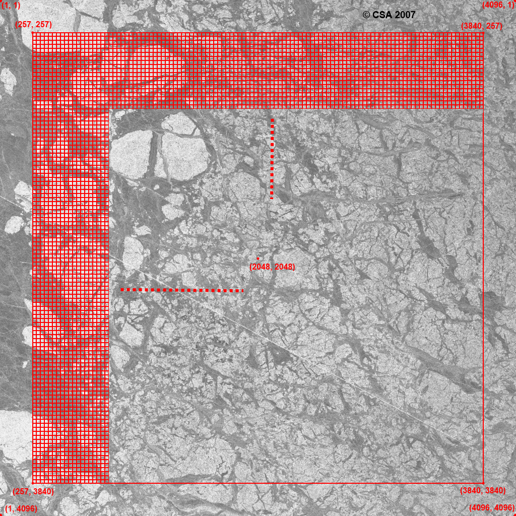
Figure 1: The motion analysis blocks superimposed on the first extracted image segment. The image is scaled down by a factor of 4. For clarity, the blocks themselves are not scaled down, so they are still 8 pixels x 8 pixels. The important points are displayed in image coordinates.
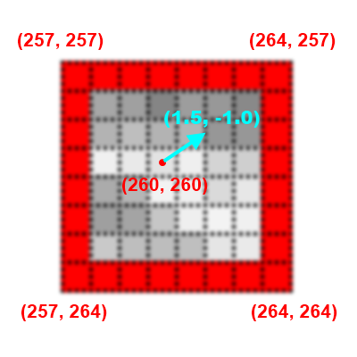
Figure 2: A single motion analysis block, enlarged for clarity. Each square represents a single pixel. The block size is 8 pixels x 8 pixels. The important points are displayed in image coordinates, with the assumption that the block is at the top left corner of the grid. The displacement vector itself is arbitrarily chosen for this example and displayed in image coordinates.
After the displacement field is calculated, the discontinuities are estimated. Discontinuities are useful for identifying long, continuous leads, cracks and ridges in the ice in the images. Conditions for discontinuity are estimated from the following method:
- The invariant shear distribution is calculated on the displacement field.
- The distribution of the resulting shear values is computed using a histogram of 1000 bins. Lower values are towards the left, and higher values are towards the right of the histogram.
- The bins are marked from left to right until the total number of values in the marked bins exceeds 95% of the total number of shear values. In effect, this process marks the smallest 95% of all shear values.
- The shear threshold (also called the noise threshold or the computed uncertainty) is set to the maximum shear value in the marked bins. Note that the shear threshold is being calculated anew for each image pair (for each displacement field).
- Every location where the shear value exceeds the shear threshold is marked as a discontinuity. In effect, this process marks the largest 5% of all shear values.
Further details on calculating the shear distribution can be found in Chapter 6 in Thomas (2009).
If the estimated displacement magnitude is small, the computed shear can be very noisy. This is observable as a large number of false positives spread across the image. Therefore, we perform noise filtering to reduce these outliers. The hypothesis for this noise filtering is that real discontinuities would cover large connected neighborhoods, while the outliers tend to cover smaller areas. This process was implemented as follows:
- The discontinuity locations are classified into patches based on their image coordinates. A patch is defined to be a collection of pixels having 8-connectivity among them. That is, if two discontinuity pixels are neighbors horizontally, vertically, or diagonally, then they belong to the same patch.
- The area (number of pixels) of each discontinuity patch is calculated.
- The distribution of the resulting area values is computed using a histogram of 200 bins. Lower values are towards the left, and higher values are towards the right of the histogram.
- The bins are marked from left to right until the total number of values in the marked bins exceeds 90% of the total number of area values. In effect, this process marks the smallest 90% of all area values.
- The area threshold is set to the maximum area value in the marked bins. Note that the area threshold is being calculated anew for each image pair (for each displacement field).
- Every discontinuity patch whose area is less than the area threshold is eliminated. All other patches are still marked as discontinuities. In effect, this process marks the largest 5% of all area values. Every pixel location residing in these large patches is regarded as a discontinuity.
Pairs with consecutive images
Each of these filenames starts with "PairM_N", where "M" and "N" indicate two image reference numbers found in Radarsat.Nominal.txt. The two images are consecutive in the time sequence. Some image pairs have not been analyzed due to one of two reasons:
- Pair30_31 and Pair31_32 have not been analyzed because the buoy was too close to one of the borders of image 31. There was not enough image data around the buoy to analyze the motion. The motion tracking system was unable to create a sufficiently-large image analysis buffer to process the image.
- Pair1_2, Pair2_3 and Pair51_52 have not been analyzed because the image time stamp >= the buoy time stamp. The archive was lacking an image before the buoy.
- PairM_N.motionsummary.txt: All motion information generated by the motion analysis between the two extracted image segments. The file contents follow a certain format:
- PairM_N.gridstruct.txt: The coordinates used to draw the longitude and latitude grid lines onto the images. To create the grid, the maximum geographical bounding area between the two extracted image segments is decomposed into equally-spaced longitudes and equally-spaced latitudes. In our analysis, the longitudes have been sampled at 1 degree while the latitudes have been sampled at 0.5 degrees. The file contents follow a certain format:
- PairM_N.overlay1.png and PairM_N.overlay2.png: Labeled figures generated from the first and second extracted image segments in the pair, respectively. The central arrow depicts the position of the buoy and the True North direction. The arrows on the first figure represent the displacement field. For clarity, the displacement field is sampled at every 16th block, both horizontally and vertically. The red markings on the first figure show the discontinuities. This overlaid data is generated from PairM_N.motionsummary.txt and PairM_N.gridstruct.txt.
- PairM_N.output.txt: The displacement values are used for drawing the Line Integral Convolution (LIC) image that represents the displacement between the two extracted image segments. LIC images are useful for visualizing high-resolution flow fields. The LIC technique approximates the flow at each grid location in a 2D flow field by iteratively stepping in the forward and backward direction. This approximation of the streamline is convolved with a texture of uniform random noise. The convolution generates a textural pattern that is highly correlated to the local direction of the flow but uncorrelated to the orthogonal direction. Essentially, this process smears the noise pattern by the vectors in the vector flow field. In our analysis, the streamlines are generated using an adaptive Runga-Kutta scheme, based on the displacement field between the two extracted image segments. For more details, see Chapter 4.2, Chapter 10 and Appendix B.2.7 in Thomas (2009). The file contents follow a certain format:
- PairM_N.lic.png: The labeled Line Integral Convolution (LIC) image that depicts the displacement between the two extracted image segments. This image is generated from PairM_N.output.txt. The central arrow depicts the position of the buoy and the True North direction. The arrows on the image represent the displacement field and clarify the direction of the flow. For clarity, the displacement field is sampled at every 16th block, both horizontally and vertically. The red markings on the image show the discontinuities. This overlaid data is generated from PairM_N.motionsummary.txt and PairM_N.gridstruct.txt.
Pairs with non-consecutive images
If the estimated displacement magnitudes obtained from consecutive images are small, it can be hard to identify discontinuities. Images that are further apart in the time sequence tend to give clearer discontinuities. Therefore, we produced additional motion analysis results from pairs where the two images were separated by 3 intermediate images in the time sequence. The resulting files have the same descriptions as those with consecutive images. However, each of these filenames starts with "PairM_N.gap3" instead of "PairM_N". Some image pairs have not been analyzed due to one of two reasons:
- Pair27_31 and Pair31_35 have not been analyzed because the buoy was too close to one of the borders of image 31. There was not enough image data around the buoy to analyze the motion. The motion tracking system was unable to create a sufficiently-large image analysis buffer to process the image.
- Pair1_5, Pair2_6 and Pair48_52 have not been analyzed because the image time stamp >= the buoy time stamp. The archive was lacking an image before the buoy.
© UD VIMS 2010